Counting triangles with SPARQL vs NetworkX

Before we begin, I should disclose: I am not a believer in the semantic web. I am not excited by the promise of linked data.

As I mentioned when I was getting started with SPARQL a few posts ago, I’ve been convinced to give this a try because Cray, Inc. has a new type of computer and this may be the lowest-overhead way for me to use it for global health metrics.

With that out of the way, here is one way that I may test drive their machine: counting triangles in massive graphs. I’ll abbreviate the introduction, counting triangles is an area that there has been a fair amount of work on in the last decade. Google scholar can get you more up-to-date than I, although I was looking into this matter towards the end of my post-doc at Microsoft Research. It is a good simplification of a more general subgraph counting challenge, and it can probably be justified in its own right as a metric of “cohesion” in social networks.

Another appealing aspect of triangle counting is that it is easily done with the Python NetworkX package:

import networkx as nx
G = nx.random_graphs.barabasi_albert_graph(10000, 5)
print 'Top ten triangles per vertex:',
print sorted(nx.triangles(G).values(), reverse=True)[:10]

It is not as easy, but also not much harder to count triangles per vertex in SPARQL (once you figure out how to transfer a graph from Python to a SPARQL server):

SELECT ?s (COUNT(?o) as ?hist)
WHERE { ?s  ?p  ?o . 
        ?o  ?p  ?oo .
        ?s  ?p  ?oo .
      }
GROUP BY ?s
ORDER BY DESC(?hist) LIMIT 10

I compared the speed of these approaches for a range of graph sizes, but just using the Jena Fuseki server for the SPARQL queries. Presumably, the Cray uRiKa will be much faster. I look forward to finding out!

time_ratio

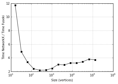
NetworkX is faster than Fuseki, 2-4x faster. But more important is the next plot, showing that both seem to take time super-linear in instance size, possibly with different exponents:
time_2

Comments Off on Counting triangles with SPARQL vs NetworkX

Filed under machine learning

Classic EM in Python: Multinomial sampling

In the classic paper on the EM algorithm, the extensive example section begins with a multinomial modeling example that is theoretically very similar to the warm-up problem on 197 animals:

We can think of the complete data as an n \times p matrix x whose (i,j) element is unity if the i-th unit belongs in the j-th of p possible cells, and is zero otherwise. The i-th row of x contains p-1 zeros and one unity, but if the i-th unit has incomplete data, some of the indicators in the i-th row of x are observed to be zero, while the others are missing and we know only that one of them must be unity. The E-step then assigns to the missing indicators fractions that sum to unity within each unit, the assigned values being expectations given the current estimate of \phi. The M-step then becomes the usual estimation of \phi from the observed and assigned values of the indicators summed over the units.

In practice, it is convenient to collect together those units with the same pattern of missing indicators, since the filled in fractional counts will be the same for each; hence one may think of the procedure as filling in estimated counts for each of the missing cells within each group of units having the same pattern of missing data.

When I first made some data to try this out, it looked like this:

import pymc as mc, numpy as np, pandas as pd, random

n = 100000
p = 5

pi_true = mc.rdirichlet(np.ones(p))
pi_true = np.hstack([pi_true, 1-pi_true.sum()])
x_true = mc.rmultinomial(1, pi_true, size=n)

x_obs = array(x_true, dtype=float)
for i in range(n):
    for j in random.sample(range(p), 3):
        x_obs[i,j] = np.nan

At first, I was pretty pleased with myself when I managed to make a PyMC model and an E-step and M-step that converged to something like the true value of \pi. The model is not super slick:

pi = mc.Uninformative('pi', value=np.ones(p)/p)

x_missing = np.isnan(x_obs)
x_initial = x_obs.copy()
x_initial[x_missing] = 0.
for i in range(n):
    if x_initial[i].sum() == 0:
        j = np.where(x_missing[i])[0][0]
        x_initial[i,j] = 1.
@mc.stochastic
def x(pi=pi, value=x_initial):
    return mc.multinomial_like(value, 1, pi)

@mc.observed
def y(x=x, value=x_obs):
    if np.allclose(x[~x_missing], value[~x_missing]):
        return 0
    else:
        return -np.inf

And the E-step/M-step parts are pretty simple:

def E_step():
    x_new = array(x_obs, dtype=float)
    for i in range(n):
        if x_new[i, ~x_missing[i]].sum() == 0:
            conditional_pi_sum = pi.value[x_missing[i]].sum()
            for j in np.where(x_missing[i])[0]:
                x_new[i,j] = pi.value[j] / conditional_pi_sum
        else:
            x_new[i, x_missing[i]] = 0.
    x.value = x_new

def M_step():
    counts = x.value.sum(axis=0)
    pi.value = (counts / counts.sum())

But the way the values converge does look nice:
em

The thing that made me feel silly was comparing this fancy-pants approach to the result of averaging all of the non-empty cells of x_obs:

ests = pd.DataFrame(dict(pr=pi_true, true=x_true.mean(0),
                    naive=pd.DataFrame(x_obs).mean(), em=pi.value),
                    columns=['pr', 'true', 'naive', 'em']).sort('true')
print np.round_(ests, 3)
      pr   true  naive     em
2  0.101  0.101  0.100  0.101
0  0.106  0.106  0.108  0.108
3  0.211  0.208  0.209  0.208
1  0.269  0.271  0.272  0.271
4  0.313  0.313  0.314  0.313

Simple averages are just as good as EM, for the simplest distribution I could think of based on the example, anyways.

To see why this EM business is worth the effort requires a more elaborate model of missingness. I made one, but it is a little bit messy. Can you make one that is nice and neat?

Comments Off on Classic EM in Python: Multinomial sampling

Filed under statistics, Uncategorized

Before getting started with the Semantic Web

I mentioned the websearching difficulty I found when getting started with Semantic Web recently, but there was one good lead I found: an O’Reilly book called Learning SPARQL, and associated blog by author Bob DuCharme. I was particularly interested in an essay on the culture gap between Semantic Web and Big Data.

I can’t believe I just said I’m particularly interested in an essay about databases!

Comments Off on Before getting started with the Semantic Web

Filed under machine learning

Getting started with the Semantic Web

I’ve been getting started with a new project, for which I need to get up to speed on this whole semantic web/linked data business. I was as let down by the results of my websearching as I was elevated by the tagged-and-up-voted material on Stack Overflow. Here is a little link library:

Why am I doing this? Because supercomputer company Cray, Inc. has built a new type of supercomputer which is optimized for graph searching, and searching RDF with SPARQL is a low-overhead way to use it. And they are running a contest for scientists to do something interesting with their new tool, in which I am a contestant.

3 Comments

Filed under machine learning

Classic EM in Python: Warm-up problem of 197 animals in PyMC

The classic paper on the EM algorithm begins with a little application in multinomial modeling:

Rao (1965, pp. 368-369) presents data in which 197 animals are distributed multinomially into four categories, so that the observed data consist of y = (y_1, y_2, y_3, y_4) = (125, 18, 20, 34).

A genetic model for the population specifies cell probabilities \left(\frac12 + \frac14\pi, \frac14(1-\pi), \frac14(1 -\pi), \frac14\pi\right) for some \pi with 0\leq \pi \leq 1.

Solving this analytically sounds very much like a 1960’s pastime to me (answer: \pi = \frac{15 + \sqrt{53809}}{394}), and a modern computer with PyMC can make short work of numerically approximating this maximum likelihood estimation. It takes no more than this:

import pymc as mc, numpy as np

pi = mc.Uniform('pi', 0, 1)
y = mc.Multinomial('y', n=197, 
                   p=[.5 + .25*pi, .25*(1-pi), .25*(1-pi), .25*pi],
                   value=[125, 18, 20, 34], observed=True)

mc.MAP([pi,y]).fit()
print pi.value

But the point is to warm-up, not to innovate. The EM way is to introduce a latent variable x = (x_1, x_2, x_3, x_4, x_5) and set y_1 = x_1+x_2, y_2=x_3, y_3=x_4, y_4=x_5, and work with a multinomial distribution for x that induces the multinomial distribution above on y. The art is determining a good latent variable, mapping, and distribution, and “good” is meant in terms of the computation it yields:

import pymc as mc, numpy as np

pi = mc.Uniform('pi', 0, 1)

@mc.stochastic
def x(n=197, p=[.5, .25*pi, .25*(1-pi), .25*(1-pi), .25*pi], value=[125.,0.,18.,20.,34.]):
    return mc.multinomial_like(np.round_(value), n, p)

@mc.observed
def y(x=x, value=[125, 18, 20, 34]):
    if np.allclose([x[0]+x[1], x[2], x[3], x[4]], value):
        return 0
    else:
        return -np.inf

It is no longer possible to get a good fit to an mc.MAP object for this model (why?), but EM does not need to. The EM approach is to alternate between two steps:

  • Update x (E-step, because it is set to its conditional expectation based on the current value of \pi)
  • Update \pi (M-step, because it is chosen to maximize the likelihood for the current value of x)

This is simply implemented in PyMC and quick to get the goods:

def E_step():
    x.value = [125 * .5 / (.5 + .25*pi.value), 125 * .25*pi.value / (.5 + .25*pi.value), 18, 20, 34]
def M_step():
    pi.value = (x.value[1] + 34.) / (x.value[1] + 34. + 18. + 20.)
for i in range(5):
    print 'iter %2d: pi=%0.4f, X=%s' %(i, pi.value, x.value)
    E_step()
    M_step()

It is not fair to compare speeds without making both run to the same tolerance, but when that is added EM is 2.5 times faster. That could be important sometimes, I suppose.

1 Comment

Filed under statistics

What is “hello, world” for statistical graphics?

Tell me on cross-validated.

1 Comment

Filed under dataviz

Rewind Data Augmentation to EM

The original paper on Data Augmentation (DA) got me thinking it was time to have a careful look at the original paper on EM. These are both highly cited papers, and Google scholar says the DA paper has been cited 2538 times (a lot!) and the EM paper has been cited 31328 times (is that possible?).

EM (which stands of Expectation-Maximization) is something I have heard about a lot, and, as an algorithm, it is even something I understood when I read a blog post relating it to a clustering algorithm that I now cannot find (maybe on the Geomblog). The arguments from the EM to DA paper, which I read recently, makes me think that there is something more than the algorithm going on here. In this later paper, Tanner and Wong identify the importance of Section 4 of the EM paper, which provides a collection of example applications of their EM algorithm. Is there something about this way of thinking that is even more important than the algorithm itself?

Comments Off on Rewind Data Augmentation to EM

Filed under statistics

What is data augmentation?

I’ve started summarizing papers for MathSciNet again, a strangely arcane practice coordinated by the American Mathematical Society. MathSciNet is a vast database of short reviews of math publications, and I loved it when I was writing the background sections of my graduate thesis. It was so useful then that I’m compelled to write summaries for it now, if I can make the time. Like reviewing, it makes me read a range of recent papers, but unlike reviewing, I don’t need to make a fuss about things that seem wrong. Fun.

I used to get to read some of the latest and greatest results in random graphs this way, but since I started up again, I’ve adjusted my preferences to receive some latest and greatest results in statistical computation. Hence my new appreciation for “data augmentation”, a term that doesn’t seem like good branding to me, but might be the key to MCMC coming into vogue for Bayesian computation.

Here is a little research list for my future self to investigate further:

1 Comment

Filed under statistics

IHME PBF application announcement

Calling recent college grads:

The Institute for Health Metrics and Evaluation at the University of Washington offers a Post-Bachelor Fellowship program that combines a full-time professional position, academic research, and education with progressive on-the-job training and mentoring from a renowned group of professors. This program provides Post-Bachelor Fellows the option to pursue for a fully-funded Master of Public Health at the University of Washington. The program description and instructions on how to apply are attached.

Further information about the Post-Bachelor Fellowship program and how to apply can be found at: IHME Post-Bachelor Fellowship.

Comments Off on IHME PBF application announcement

Filed under education

GBD 2010

The massive project I’ve been working on since moving from math to global health has been published!

The Global Burden of Disease Study 2010 (GBD 2010) is the largest ever systematic effort to describe the global distribution and causes of a wide array of major diseases, injuries, and health risk factors. The results show that infectious diseases, maternal and child illness, and malnutrition now cause fewer deaths and less illness than they did twenty years ago. As a result, fewer children are dying every year, but more young and middle-aged adults are dying and suffering from disease and injury, as non-communicable diseases, such as cancer and heart disease, become the dominant causes of death and disability worldwide. Since 1970, men and women worldwide have gained slightly more than ten years of life expectancy overall, but they spend more years living with injury and illness.

GBD 2010 consists of seven Articles, each containing a wealth of data on different aspects of the study (including data for different countries and world regions, men and women, and different age groups), while accompanying Comments include reactions to the study’s publication from WHO Director-General Margaret Chan and World Bank President Jim Yong Kim. The study is described by Lancet Editor-in-Chief Dr Richard Horton as “a critical contribution to our understanding of present and future health priorities for countries and the global community.”

Now I have to get my book about the methods out the door as well…

2 Comments

Filed under global health