Tag Archives: statistics

G.E.P. Box on Model Building

The Edward library http://edwardlib.org/ has made the modeling approach of G.E.P. Box sound appealing to me. Here is some reading on it:

https://www.jstor.org/stable/1266570?seq=1#page_scan_tab_contents
https://www.jstor.org/stable/1266125?seq=1#page_scan_tab_contents
https://www.jstor.org/stable/1266318?seq=1#page_scan_tab_contents
https://www.jstor.org/stable/2286841?seq=1#page_scan_tab_contents
https://www.jstor.org/stable/2982063?seq=1#page_scan_tab_contents

Comments Off on G.E.P. Box on Model Building

Filed under Uncategorized

ML vs Stats

What is the difference between machine learning and statistics? Can it be captured in a tweet?

1 Comment

Filed under education

Tukey quote I half-remembered

I was trying to remember some quote by the exploratory data analysis master John Tukey yesterday, and I think this is it:

No catalog of techniques can convey a willingness to look for what can be seen, whether or not anticipated. Yet this is at the heart of exploratory data analysis. The graph paper—and transparencies—are there, not as a technique, but rather as a recognition that the picture-examining eye is the best finder we have of the wholly unanticipated.

It is from John W. Tukey, We Need Both Exploratory and Confirmatory, The American Statistician, Vol. 34, No. 1 (Feb., 1980), pp. 23-25.

I remembered a version about the visual cortex as a the most advance signal processing device, so maybe there is another version of this out there.

Comments Off on Tukey quote I half-remembered

Filed under statistics

Parameterizing Negative Binomial distributions

The negative binomial distribution is cool. Sometimes I think that.

Sometimes I think it is more trouble than it’s worth, a complicated mess.

Today, both.

Wikipedia and PyMC parameterize it differently, and it is a source of continuing confusion for me, so I’m just going to write it out here and have my own reference. (Which will match with PyMC, I hope!)

The important thing about the negative binomial, as far as I’m concerned, is that it is like a Poisson distribution, but “over-dispersed”. That is to say that the standard deviation is not always the square root of the mean. So I’d like to parameterize it with a parameter \mu for the mean and \delta for the dispersion. This is almost what PyMC does, except it calls the dispersion parameter \alpha instead of \delta.

The slightly less important, but still informative, thing about the negative binomial, as far as I’m concerned, is that the way it is like a Poisson distribution is very direct. A negative binomial is a Poisson that has a Gamma-distributed random variable for its rate. In other words (symbols?), Y \sim \text{NegativeBinomial}(\mu, \delta) is just shorthand for

Y \sim \text{Poisson}(\lambda),
\lambda \sim \text{Gamma}(\mu, \delta).

Unfortunately, nobody parameterizes the Gamma distribution this way. And so things get really confusing.

The way to get unconfused is to write out the distributions, although after they’re written, you might doubt me:

The negative binomial distribution is
f(k \mid \mu, \delta) = \frac{\Gamma(k+\delta)}{k! \Gamma(\delta)} (\delta/(\mu+\delta))^\delta (\mu/(\mu+\delta))^k
and the Poisson distribution is
f(k \mid \lambda) = \frac{e^{-\lambda}\lambda^k}{k!}
and the Gamma distribution is
f(x \mid \alpha, \beta) = \frac{\beta^{\alpha}x^{\alpha-1}e^{-\beta x}}{\Gamma(\alpha)}

Hmm, does that help yet? If \alpha = \delta and \beta = \delta/\mu, it all works out:
\frac{\Gamma(k+\delta)}{\Gamma(\delta)k!} \left(\frac{\delta}{\pi+\delta}\right)^\delta \left(\frac{\pi}{\pi+\delta}\right)^k  =  \int_0^\infty \frac{e^{-\lambda}\lambda^k}{k!} \lambda^{\delta-1} e^{-\lambda \delta/\mu} \frac{(\delta/\mu)^{\delta}}{\Gamma(\delta)}d \lambda.

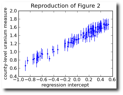
But instead of integrating it analytically (or in addition to), I am extra re-assured by seeing the results of a little PyMC model for this:

I put a notebook for making this plot in my pymc-examples repository. Love those notebooks. [pdf] [ipynb]

1 Comment

Filed under statistics

Life Expectancy by County in US

This recent study by my colleagues has been making headlines a lot last week, but I’m just getting to write about it now.  While I was busy, stories about it appeared in high-profile outlets like NPR and the Statistical Modeling, Causal Inference, and Social Science blog.

As I’ve been thinking for two years (according to the ancient post I pushed out the door yesterday), life expectancy is a weird statistic. Life expectancy at birth is not, as the name might imply, a prediction on the average length of the life of a baby born this year. It is something more complicated to describe, but easier to predict. I like to think of it as the length of life if you froze the world exactly the way it is right now, and the baby today was exposed to the mortality risk of today’s one-year-olds next year, today’s two-year-olds in two years, etc. Although, as a friend pointed out two weeks ago, this is not a really good way to look at things either, if you push the analogy too hard. Currently Wikipedia isn’t really helpful on this matter, but maybe it will be better in the future.

There is another interesting thing in this paper, which is the validation approach the authors used. Unfortunately, it’s full development is in a paper still in press. Here is what they have to say about it so far:

We validated the performance of the model by creating small counties whose “true” underlying death rates were known. We did this by treating counties with large populations (> 750,000) as those where death rates have little sampling uncertainty. We then repeatedly sampled residents and deaths from these counties (by year and sex) to construct simulated small-county populations. We used the above model to predict mortality for these small, sampled-down counties, which were then compared with the mortality of the original large county.

I believe that this is fully developed in the paper which they cite at the beginning of the modeling section, Srebotnjak T, Mokdad AH, Murray CJL: A novel framework for validating and applying standardized small area measurement strategies, submitted. From what I’ve heard about it, I like it.

Comments Off on Life Expectancy by County in US

Filed under global health

Journal Culture

All fields have their quirks in publication style. Today I’m thinking about statistics, because I’ve been asked to explain something about survey weights to our post-bachelor’s fellows. There is a nice paper on the matter by Andrew Gelman, which starts strong, with first sentence “Survey weighting is a mess.” Start like that, and you’re sure to get a response from survey statisticians, who (at least I imagine) think of themselves as about as tidy as it comes.

The quirk in stats publications that I’m thinking of today is the Comment/Rejoinder format, wherein an article was published together with responses from several statisticians who don’t all agree with the article, and then a response from authors of the article. This is cool.

Unfortunately, Google scholar hasn’t kept up with this format, and searching for the paper title Struggles with Survey Weighting and Regression Modeling found me just one of the five comments. Project Euclid hasn’t kept up either, with only a tiny link from the article to the table of contents from the journal it appeared in. And thus I was forced to follow the obscure links in the pdf of the article to find the comprehensive list, which I’m putting here in case I need to find them all again sometime.

Statistical Science, Vol. 22, No. 2
: Article/Comments/Rejoiner on Survey Weights

Comments Off on Journal Culture

Filed under statistics

9 Hours to Numeracy

I’m helping to plan an Introduction to Statistics for incoming post-bachelors fellows in the next month, and because of the wide range of backgrounds these recent college graduates will be coming from, I’m approaching it as a short course on numeracy (we’ve got about 9 hours of lecture time scheduled for it), focused on statistics. This will be complemented with a very hands-on dose of STATA, but I’m going to try not to think about that.

My favorite numeracy-in-stats book is a dusty classic, and it would have survived on its name alone: How to Lie with Statistics. I wonder if that title is too cheeky for global health applications when the numbers really matter…

Do you know this book, and do you like it? Or is there a more modern book or article that I should think of instead? What would you pack into 9 hours of stats numeracy training. Tell me.

7 Comments

Filed under education

What is this “effects” business?

I’ve got to figure out what people mean when they say “fixed effect” and “random effect”, because I’ve been confused about it for a year and I’ve been hearing it all the time lately.

Bayesian Data Analysis is my starting guide, which includes a footnote on page 391:

The terms ‘fixed’ and ‘random’ come from the non-Bayesian statistical tradition are are somewhat confusing in a Bayesian context where all unknown parameters are treated as ‘random’. The non-Bayesian view considers fixed effects to be fixed unknown quantities, but the standard procedures proposed to estimate these parameters, based on specified repeated-sampling properties, happen to be equivalent to the Bayesian posterior inferences under a noninformative (uniform) prior distribution.

That doesn’t totally resolve my confusion, though, because my doctor-economist colleagues are often asking for the posterior mean of the random effects, or similarly non-non-Bayesian sounding quantities.

I was about to formulate my working definition, and see how long I can stick to it, but then I was volunteered to teach a seminar on this very topic! So instead of doing the work now, I turn to you, wise internet, to tell me how I can understand this thing.

6 Comments

Filed under statistics

Practical MCMC Advice: When to Stop

I read some good practical advice about when enough is enough in Markov Chain Monte Carlo sampling this morning. In their “Inference from simulations and monitoring convergence” chapter of Handbook of Markov Chain Monte Carlo, Andrew Gelman and Kenneth Shirley say many useful things in a quickly digested format. Continue reading

Comments Off on Practical MCMC Advice: When to Stop

Filed under MCMC, statistics, TCS

Multilevel (hierarchical) modeling: what it can and cannot do in Python


I re-read a short paper of Andrew Gelman’s yesterday about multilevel modeling, and thought “That would make a nice example for PyMC”.  The paper is “Multilevel (hierarchical) modeling: what it can and cannot do, and R code for it is on his website.

To make things even easier for a casual blogger like myself, the example from the paper is extended in the “ARM book”, and Whit Armstrong has already implemented several variants from this book in PyMC. Continue reading

17 Comments

Filed under MCMC, statistics