
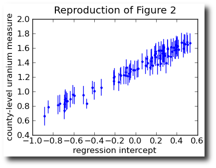
I re-read a short paper of Andrew Gelman’s yesterday about multilevel modeling, and thought “That would make a nice example for PyMC”. The paper is “Multilevel (hierarchical) modeling: what it can and cannot do, and R code for it is on his website.
To make things even easier for a casual blogger like myself, the example from the paper is extended in the “ARM book”, and Whit Armstrong has already implemented several variants from this book in PyMC.
There is really nothing left for me to do but collect up the links and find a nice graphic. I guess I’ll go the extra distance and condense the code to as few lines as possible and paste it in here, too. Here’s my github, if you want to get my reformed csv files and follow along at home.
household_data = [d for d in csv.DictReader(open('household.csv'))]
county_data = [d for d in csv.DictReader(open('county.csv'))]

# hyper-priors
g = Uniform('gamma', [0,0], [100,100])

s_a = Uniform('sigma_a', 0, 100)

# priors
a = {}
for d in county_data:
    @stochastic(name='a_%s'%d['county'])
    def a_j(value=0., g=g, u_j=float(d['u']), s_a=s_a):
        return normal_like(value, g[0] + g[1]*u_j, s_a**-2.)
    a[d['county']] = a_j

b = Uniform('beta', 0, 100)

s_y = Uniform('sigma_y', 0, 100)

# likelihood
y = {}
for d in household_data:
    @stochastic(observed=True, name='y_%s'%d['household'])
    def y_i(value=float(d['y']), a_j=a[d['county']], b=b,
            x_ij=float(d['x']), s_y=s_y):
        return normal_like(value, a_j + b*x_ij, s_y**-2.)
    y[d['household']] = y_i

mc = MCMC([g, s_a, a, b, s_y, y])
mc.sample(10000, 2500, verbose=1)

Now who’s going to race this against WinBugs?
Thanks for sharing the code. I am thinking that it would be interesting also to show some performance tests of different implementations in different programs. I have made the commitment to start doing it myself.
Anyway, thanks.
Great, Xavier! Let me know how it goes.
This took about 75 min to run on my laptop, but I bet when the pymc-users crowd gives it a look, there will be suggestions for major speedups.
Hey Xavier,
Thanks for doing this; it does make for a nice example. I would suggest a couple of fundamental structural changes from a PyMC implementation standpoint. As much as possible, you want to avoid loops, and stick with vector-valued stochastics whenever possible. Not only is the code more concise, but it is far faster. Here is my version of the multilevel_radon model; notice the use of indexing for the county intercepts.
Sorry, my embedded code snippet did not show up. Here is a link: http://pastie.org/726147
Thanks, Chris. I’ll try a laptop-melting speed test tonight, and report back.
Chris wins! 200x speed up…
Sorry — realized that I said “Hey Xavier” when I should have said “Hey Abraham”.
Not that Xavier doesn’t deserve a “hey”, but you know …
🙂
Hi Abraham,
Thanks very much for your post and sharing your code!
I’m having trouble reproducing your figure using Chris’s fast version. What I get when I run run_multilevel_radon_fast.py is shown in the following figure:
http://drp.ly/5HcbD
I’m using a recent SVN version of PyMC with NumPy v1.4.0.dev7805 on a Mac with Python 2.6. Have you verified that Chris’s fast version actually yields the right numbers?
Running your original version yields a figure identical to the one in your blog post (and identical to the results from running Gelman’s model with JAGS).
Thanks,
Todd
Hi Todd,
I think there is a small bug in Chris’s code, and I tried fixing it here:
http://github.com/aflaxman/pymc_radon/commit/b8f7c7b10cc769cf2840fa3e549d317076b24fa0#L1L16
I haven’t had time to verify it carefully, though, so it would be great if you can.
Hi Abraham,
I think I actually used the latest versions (12/10/2009, better priors, floats not ints) of multilevel_radon_fast and run_multilevel_radon_fast.py.
I’m going to spend some time this morning trying to figure out what’s going on, and I’ll let you know if I have any luck.
Todd
Oh, my other thought is to make sure you are waiting long enough for the “burn-in” period. The AdaptiveMetropolis might need 10-20K samples to learn about the shape of the probability space.
Well, it took me a little more time than I imagined to figure things out, or at least to *think* that I’ve figured things out.
It all seems to come down to initialization. The original version initializes all of the “a” (or “alpha”) values to 0, while the fast version leaves the initialization up to PyMC. After even 100 million iterations, the fast version without “thoughtful” initialization does not converge (although it’s clearly moving in the right direction).
If I initialize the stochastics following Gelman’s prescription (i.e., normal variables are initialized with random draws from a N(0, 1) distribution and uniform variables are initialized with draws from a uniform(0, 1) distribution; p. 350 of Gelman and Hill), then the fast version does converge after a still lengthy ~200,000 iterations.
It’s worth noting that JAGS, even without sensible initialization, converges in a mere few thousand iterations.
Thanks again for sharing your code!
Todd
Abraham,
Thanks for posting this example up! The model variation that gave me the most trouble is actually the inverse wishart version.
The version that I put together was miserably slow, and if I recall correctly I don’t think I was able to get identical output to Gelman’s version.
I’d be obliged if someone would have a look:
http://github.com/armstrtw/pymc_radon/blob/master/radon_inv_wishart.py
-Whit
Hi Whit,
I had some down time this morning, so I took a look. There were indeed some possible speedups, and the big one is from vectorizing the MvNormal stoch. That makes things about 15x faster.
Can you make sure that you still like the estimates coming out? As Todd discovered above, a computation completing quickly is only part of the challenge.
Pingback: 2010 in review | Healthy Algorithms