Monthly Archives: January 2013

Journal Club: Information for decision making from imperfect national data

A nice connection from last week’s journal club paper to this week’s: the errors in health information system data. Last week was about correcting the bias from missing individuals. This week is about correcting the bias from missing facilities.

From the key figure, it looks like missing individuals bias things more:

Gething et al. BMC Medicine 2007 5:37   doi:10.1186/1741-7015-5-37

1 Comment

Filed under global health

k-NN in SPARQL?

Is a SPARQL query capable of finding the k nearest neighbors for several vectors simultaneously? I don’t think so, but I’ve been wrong before. Tell me on Stack Overflow.

Comments Off on k-NN in SPARQL?

Filed under machine learning

Journal Club: Sampling-Based Approach to Determining Outcomes of Patients Lost to Follow-Up in Antiretroviral Therapy Scale-Up Programs in Africa

This week’s paper for journal club is short and has a nice figure:

Geng et al, Sampling-Based Approach to Determining Outcomes of Patients Lost to Follow-Up in Antiretroviral Therapy Scale-Up Programs in Africa
naive_and_corrected

It looks like this corrected estimate is quite different than the uncorrected version!

I think the mathematics involved have an extended treatment in this work referenced by Geng et al: Addressing an idiosyncrasy in estimating survival curves using double-sampling in the presence of self-selected right censoring

2 Comments

Filed under global health

MLK’s address to APA

Today is Martin Luther King Day in the US, a civil rights holiday. I heard a recording of this address by King to the 1967 meeting of the American Psychological Association, and then couldn’t find a copy of the text… until now, when I searched the web with two critical typos in the search terms.

The Role of the Behavioral Scientist in the Civil Rights Movement
By Martin Luther King Jr.


There are certain technical words in every academic discipline which soon become stereotypes and even clichés. Every academic discipline has its technical nomenclature. You who are in the field of psychology have given us a great word. It is the word maladjusted. This word is probably used more than any other word in psychology. It is a good word; certainly it is good that in dealing with what the word implies you are declaring that destructive maladjustment should be destroyed. You are saying that all must seek the well-adjusted life in order to avoid neurotic and schizophrenic personalities.

But on the other hand, I am sure that we will recognize that there are some things in our society, some things in our world, to which we should never be adjusted. There are some things concerning which we must always be maladjusted if we are to be people of good will. We must never adjust ourselves to racial discrimination and racial segregation. We must never adjust ourselves to religious bigotry. We must never adjust ourselves to economic conditions that take necessities from the many to give luxuries to the few. We must never adjust ourselves to the madness of militarism, and the self-defeating effects of physical violence.

(all)

Comments Off on MLK’s address to APA

Filed under general

ipython autoreloading

This will be useful.

Comments Off on ipython autoreloading

Filed under Uncategorized

Power of SPARQL?

Is a SPARQL query computationally powerful enough to test (s,t)-connectivity? I don’t think so, but I don’t understand the mysterious PropertyPath, and even without it, I’m not sure. Tell me on Stack Overflow.

1 Comment

Filed under combinatorial optimization

Journal Club is Back

Or actually, I am back. Back to facilitating the post-graduate fellowship (PGF) journal club. Here is what we are reading this week, Impact assessment of malaria vector control using routine surveillance data in Zambia: implications for monitoring and evaluation, which is a highly accessed article according to the Malaria Journal website. Is it also highly accessible? We shall see. Any wisdom on this that I can pass on to the fellows is welcome.

Figure 1. Estimated operational ITN distributions by district in Zambia from 2003–2010, representing percentage of district households receiving 3 ITNs per household (HH) in overlapping 3-year intervals (MoH, 2010).

Figure 1. Estimated operational ITN distributions by district in Zambia from 2003–2010, representing percentage of district households receiving 3 ITNs per household (HH) in overlapping 3-year intervals (MoH, 2010).

1 Comment

Filed under global health

Counting triangles with SPARQL vs NetworkX

Before we begin, I should disclose: I am not a believer in the semantic web. I am not excited by the promise of linked data.

As I mentioned when I was getting started with SPARQL a few posts ago, I’ve been convinced to give this a try because Cray, Inc. has a new type of computer and this may be the lowest-overhead way for me to use it for global health metrics.

With that out of the way, here is one way that I may test drive their machine: counting triangles in massive graphs. I’ll abbreviate the introduction, counting triangles is an area that there has been a fair amount of work on in the last decade. Google scholar can get you more up-to-date than I, although I was looking into this matter towards the end of my post-doc at Microsoft Research. It is a good simplification of a more general subgraph counting challenge, and it can probably be justified in its own right as a metric of “cohesion” in social networks.

Another appealing aspect of triangle counting is that it is easily done with the Python NetworkX package:

import networkx as nx
G = nx.random_graphs.barabasi_albert_graph(10000, 5)
print 'Top ten triangles per vertex:',
print sorted(nx.triangles(G).values(), reverse=True)[:10]

It is not as easy, but also not much harder to count triangles per vertex in SPARQL (once you figure out how to transfer a graph from Python to a SPARQL server):

SELECT ?s (COUNT(?o) as ?hist)
WHERE { ?s  ?p  ?o . 
        ?o  ?p  ?oo .
        ?s  ?p  ?oo .
      }
GROUP BY ?s
ORDER BY DESC(?hist) LIMIT 10

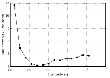
I compared the speed of these approaches for a range of graph sizes, but just using the Jena Fuseki server for the SPARQL queries. Presumably, the Cray uRiKa will be much faster. I look forward to finding out!

time_ratio

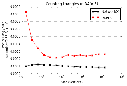
NetworkX is faster than Fuseki, 2-4x faster. But more important is the next plot, showing that both seem to take time super-linear in instance size, possibly with different exponents:
time_2

Comments Off on Counting triangles with SPARQL vs NetworkX

Filed under machine learning

Classic EM in Python: Multinomial sampling

In the classic paper on the EM algorithm, the extensive example section begins with a multinomial modeling example that is theoretically very similar to the warm-up problem on 197 animals:

We can think of the complete data as an n \times p matrix x whose (i,j) element is unity if the i-th unit belongs in the j-th of p possible cells, and is zero otherwise. The i-th row of x contains p-1 zeros and one unity, but if the i-th unit has incomplete data, some of the indicators in the i-th row of x are observed to be zero, while the others are missing and we know only that one of them must be unity. The E-step then assigns to the missing indicators fractions that sum to unity within each unit, the assigned values being expectations given the current estimate of \phi. The M-step then becomes the usual estimation of \phi from the observed and assigned values of the indicators summed over the units.

In practice, it is convenient to collect together those units with the same pattern of missing indicators, since the filled in fractional counts will be the same for each; hence one may think of the procedure as filling in estimated counts for each of the missing cells within each group of units having the same pattern of missing data.

When I first made some data to try this out, it looked like this:

import pymc as mc, numpy as np, pandas as pd, random

n = 100000
p = 5

pi_true = mc.rdirichlet(np.ones(p))
pi_true = np.hstack([pi_true, 1-pi_true.sum()])
x_true = mc.rmultinomial(1, pi_true, size=n)

x_obs = array(x_true, dtype=float)
for i in range(n):
    for j in random.sample(range(p), 3):
        x_obs[i,j] = np.nan

At first, I was pretty pleased with myself when I managed to make a PyMC model and an E-step and M-step that converged to something like the true value of \pi. The model is not super slick:

pi = mc.Uninformative('pi', value=np.ones(p)/p)

x_missing = np.isnan(x_obs)
x_initial = x_obs.copy()
x_initial[x_missing] = 0.
for i in range(n):
    if x_initial[i].sum() == 0:
        j = np.where(x_missing[i])[0][0]
        x_initial[i,j] = 1.
@mc.stochastic
def x(pi=pi, value=x_initial):
    return mc.multinomial_like(value, 1, pi)

@mc.observed
def y(x=x, value=x_obs):
    if np.allclose(x[~x_missing], value[~x_missing]):
        return 0
    else:
        return -np.inf

And the E-step/M-step parts are pretty simple:

def E_step():
    x_new = array(x_obs, dtype=float)
    for i in range(n):
        if x_new[i, ~x_missing[i]].sum() == 0:
            conditional_pi_sum = pi.value[x_missing[i]].sum()
            for j in np.where(x_missing[i])[0]:
                x_new[i,j] = pi.value[j] / conditional_pi_sum
        else:
            x_new[i, x_missing[i]] = 0.
    x.value = x_new

def M_step():
    counts = x.value.sum(axis=0)
    pi.value = (counts / counts.sum())

But the way the values converge does look nice:
em

The thing that made me feel silly was comparing this fancy-pants approach to the result of averaging all of the non-empty cells of x_obs:

ests = pd.DataFrame(dict(pr=pi_true, true=x_true.mean(0),
                    naive=pd.DataFrame(x_obs).mean(), em=pi.value),
                    columns=['pr', 'true', 'naive', 'em']).sort('true')
print np.round_(ests, 3)
      pr   true  naive     em
2  0.101  0.101  0.100  0.101
0  0.106  0.106  0.108  0.108
3  0.211  0.208  0.209  0.208
1  0.269  0.271  0.272  0.271
4  0.313  0.313  0.314  0.313

Simple averages are just as good as EM, for the simplest distribution I could think of based on the example, anyways.

To see why this EM business is worth the effort requires a more elaborate model of missingness. I made one, but it is a little bit messy. Can you make one that is nice and neat?

Comments Off on Classic EM in Python: Multinomial sampling

Filed under statistics, Uncategorized

Before getting started with the Semantic Web

I mentioned the websearching difficulty I found when getting started with Semantic Web recently, but there was one good lead I found: an O’Reilly book called Learning SPARQL, and associated blog by author Bob DuCharme. I was particularly interested in an essay on the culture gap between Semantic Web and Big Data.

I can’t believe I just said I’m particularly interested in an essay about databases!

Comments Off on Before getting started with the Semantic Web

Filed under machine learning