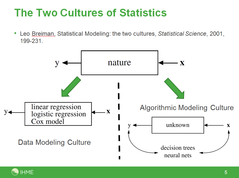
A nice example of using PyMC for multilevel (aka “Random Effects”) modeling came through on the PyMC mailing list a couple of weeks ago, and I’ve put it into a git repo so that I can play around with it a little, and collect up the feedback that the list generates.
Here is the situation:
Hi All,
New to this group and to PyMC (and mostly new to Python). In any case, I’m writing to ask for help in specifying a multilevel model (mixed model) for what I call partially clustered designs. An example of a partially clustered design is a 2-condition randomized psychotherapy study where subjects are randomly assigned to conditions. In condition 1, subjects are treated in small groups of say 8 people a piece. In the condition 2, usually a control, subjects are only assessed on the outcome (they don’t receive an intervention). Thus you have clustering in condition 1 but not condition 2.
The model for a 2-condition study looks like (just a single time point to keep things simpler):

where y_ij is the outcome for the ith person in cluster j (in most multilevel modeling software and in PROC MCMC in SAS, subjects in the unclustered condition are all in clusters of just 1 person), b_0 is the overall intercept, b_1 is the treatment effect, Tx is a dummy coded variable coded as 1 for the clustered condition and 0 for the unclustered condition, u_j is the random effect for cluster j, and e_ij is the residual error. The variance among clusters is \sigma^2_u and the residual term is \sigma^2_e (ideally you would estimate a unique residual by condition).
Because u_j interacts with Tx, the random effect is only contributes to the clustered condition.
In my PyMC model, I expressed the model in matrix form – I find it easier to deal with especially for dealing with the cluster effects. Namely:
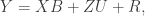
where X is an n x 2 design matrix for the overall intercept and intervention effect, B is a 1 x 2 matrix of regression coefficients, Z is an n x c design matrix for the cluster effects (where c is equal to the number of clusters in the clustered condition), and U is a c x 1 matrix of cluster effects. The way I’ve written the model below, I have R as an n x n diagonal matrix with \sigma^2_e on the diagonal and 0’s on the off-diagonal.
All priors below are based on a model fit in PROC MCMC in SAS. I’m trying to replicate the analyses in PyMC so I don’t want to change the priors.
The data consist of 200 total subjects. 100 in the clustered condition and 100 in the unclustered. In the clustered condition there are 10 clusters of 10 people each. There is a single outcome variable.
I have 3 specific questions about the model:
- Given the description of the model, have I successfully specified the model? The results are quite similar to PROC MCMC, though the cluster variance (\sigma^2_u) differs more than I would expect due to Monte Carlo error. The differences make me wonder if I haven’t got it quite right in PyMC.
-
Is there a better (or more efficient) way to set up the model? The model runs quickly but I am trying to learn Python and to get better at optimizing how to set up models (especially multilevel models).
-
How can change my specification so that I can estimate unique residual variances for clustered and unclustered conditions? Right now I’ve estimated just a single residual variance. But I typically want separate estimates for the residual variances per intervention condition.
Here are my first responses:
1. This code worked for me without any modification. 🙂 Although when
I tried to run it twice in the same ipython session, it gave me
strange complaints. (for pymc version 2.1alpha, wall time 78s).
For the newest version in the git repo (pymc version 2.2grad,
commit ca77b7aa28c75f6d0e8172dd1f1c3f2cf7358135, wall time 75s) it
didn’t complain.
2. I find the data wrangling section of the model quite opaque. If
there is a difference between the PROC MCMC and PyMC results, this
is the first place I would look. I’ve been searching for the most
transparent ways to deal with data in Python, so I can share some
of my findings as applied to this block of code.
3. The model could probably be faster. This is the time for me to
recall the two cardinal rules of program optimization: 1) Don’t
Optimize, and 2) (for experts only) Don’t Optimize Yet.
That said, the biggest change to the time PyMC takes to run is in
the step methods. But adjusting this is a delicate operation.
More on this to follow.
4. Changing the specification is the true power of the PyMC approach,
and why this is worth the extra effort, since a random effects
model like yours is one line of STATA. So I’d like to write out
in detail how to change it. More on this to follow.
5. Indentation should be 4 spaces. Diverging from this inane detail
will make python people itchy.
Have a look in the revision history and the git repo README for more.
Good times. Here is my final note from the time I spent messing around:
Django and Rails have gotten a lot of mileage out of emphasizing
_convention_ in frequently performed tasks, and I think that PyMC
models could also benefit from this approach. I’m sure I can’t
develop our conventions myself, but I have changed all the file names
to move towards what I think we might want them to look like. Commit
linked here.
My analyses often have these basic parts: data, model, fitting code,
graphics code. Maybe your do, too.
p.s. Scott and I have started making an automatic model translator, to generate models like this from the kind of concise specification that users of R and STATA are familiar with. More news on that in a future post.

 for the mean and
  for the dispersion. This is almost what PyMC does, except it calls the dispersion parameter
  instead of
  is just shorthand for
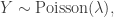


 and
and  , it all works out: