Tag Archives: pymc

MCMC in Python: Part IIb of PyMC Step Methods and their pitfalls

Two weeks ago, I slapped together a post about the banana distribution and some of my new movies sampling from it. Today I’m going to explore the performance of MCMC with the Adaptive Metropolis step method when the banana dimension grows and it becomes more curvy.

To start things off, have a look at the banana model, as implemented for PyMC:

    C_1 = pl.ones(dim)
    C_1[0] = 100.
    X = mc.Uninformative('X', value=pl.zeros(dim))

    def banana_like(X, tau, b):
        phi_X = pl.copy(X)
        phi_X *= 30. # rescale X to match scale of other models
        phi_X[1] = phi_X[1] + b*phi_X[0]**2 - 100*b

        return mc.normal_like(phi_X, 0., tau)

    @mc.potential
    def banana(X=X, tau=C_1**-1, b=b):
        return banana_like(X, tau, b)

Pretty simple stuff, right? This is a pattern that I find myself using a lot, an uninformative stochastic variable that has the intended distribution implemented as a potential. If I understand correctly, it is something that you can’t do easily with BUGS.

Adaptive Metropolis is (or was) the default step method that PyMC uses to fit a model like this, and you can ensure that it is used (and fiddle with the AM parameters) with the use_step_method() function:

mod.use_step_method(mc.AdaptiveMetropolis, mod.X)

Important Tip: If you want to experiment with different step methods, you need to call mod.use_step_method() before doing any sampling. When you call mod.sample(), any stochastics without step methods assigned are given the method that PyMC deems best, and after they are assigned, use_step_method adds additional methods, but doesn’t remove the automatically added ones. (See this discussion from PyMC mailing list.)

So let’s see how this Adaptive Metropolis performs on a flattened banana as the dimension increases:

You can tell what dimension the banana lives in by counting up the panels in the autocorrelation plots in the upper right of each video, 2, 4 or 8. Definitely AM is up to the challenge of sampling from an 8-dimensional “flattened banana”, but this is nothing more than an uncorrelated normal distribution that has been stretched along one axis, so the results shouldn’t impress anyone.

Here is what happens in a more curvy banana:

Now you can see the performance start to degrade. AM does just fine in a 2-d banana, but its going to need more time to sample appropriately from a 4-d one and even more for the 8-d. This is similar to the way a cross-diagonal region breaks AM, but a lot more like something that could come up in a routine statistical application.

For a serious stress test, I can curve the banana even more:

Now AM has trouble even with the two dimensional version.

I’ve had an idea to take this qualitative exploration and quantify it to do a real “experimental analysis of algorithms” -style analysis. Have you seen something like this already? I do have enough to do without making additional work for myself.

Comments Off on MCMC in Python: Part IIb of PyMC Step Methods and their pitfalls

Filed under statistics, TCS

MCMC in Python: Part II of PyMC Step Methods and their pitfalls

I had a good time with the first round of my Step Method Pitfalls: besides making some great movies, I got a tip on how to combine Hit-and-Run with Adaptive Metropolis (together they are “the H-RAM“, fitting since the approach was suggested by Aram). And even more important than getting the tip, I did enough of a proof-of-concept to inspire Anand to rewrite it in the correct PyMC style. H-RAM lives.

Enter the GHME, where I had a lot of good discussions about methods for metrics, and where Mariel Finucane told me that her stress test for new step methods is always the banana (from Haario, Saksman, Tamminen, Adaptive proposal distribution for random walk Metropolis algorithm, Computational Statistics 1999):

The non-linear banana-shaped distributions are constructed from the Gaussian ones by ‘twisting’ them as follows. Let f be
the density of the multivariate normal distribution N(0, C_1) with the covariance again given by C_1 = {\rm diag}(100, 1, ..., 1). The density function of the ‘twisted’ Gaussian with the nonlinearity parameter b > 0 is given by f_b = f \circ \phi_b, where the function \phi_b(x) = (x_1, x_2 + b x_1^2 - 100b, x_3, ..., x_n).

It’s a good distribution, and it makes for a good movie.

More detailed explorations to follow. What do you want to see?

1 Comment

Filed under statistics, TCS

Gaussian Processes and Jigsaw Puzzles with PyMC.gp

I was thinking about cutting something up into little pieces the other day, let’s not get into the details. The point is, I turned my destructive urge into creative energy when I started thinking about jigsaw puzzles. You might remember when my hobby was maze making with randomly generated bounded depth spanning trees a few months ago. It turns out that jigsaw puzzles are just as fun.

The secret ingredient to my jigsaw puzzle design is the Gaussian process with a Matern covariance function. (Maybe you knew that was coming.) GPs are an elegant way to make the little nubs that hold the puzzle together. It’s best to use two of them together to make the nub, like this:

Doing this is not hard at all, once you sort out the intricacies of the PyMC.gp package, and takes only a few lines of Python code:

def gp_puzzle_nub(diff_degree=2., amp=1., scale=1.5, steps=100):
    """ Generate a puzzle nub connecting point a to point b"""

    M, C = uninformative_prior_gp(0., diff_degree, amp, scale)
    gp.observe(M, C, data.puzzle_t, data.puzzle_x, data.puzzle_V)
    GPx = gp.GPSubmodel('GP', M, C, pl.arange(1))
    X = GPx.value.f(pl.arange(0., 1.0001, 1. / steps))

    M, C = uninformative_prior_gp(0., diff_degree, amp, scale)
    gp.observe(M, C, data.puzzle_t, data.puzzle_y, data.puzzle_V)
    GPy = gp.GPSubmodel('GP', M, C, pl.arange(1))
    Y = GPy.value.f(pl.arange(0., 1.0001, 1. / steps))
    
    return X, Y

(full code here)

I was inspired by something Andrew Gelman blogged, about the utility of writing a paper and a blog post about this or that. So I tried it out. It didn’t work for me, though. There isn’t a paper’s worth of ideas here, but now I’ve depleted my energy before finishing the blog. Here it is: an attempted paper to accompany this post. Patches welcome.

In addition to a aesthetically pleasing diversion, I also got something potentially useful out of this, a diagram of how misspecifying any one of the parameters of the Matern covariance function can lead to similarly strange looking results. This is my evidence that you can’t tell if your amplitude is too small or your scale is too large from a single bad fit:

Comments Off on Gaussian Processes and Jigsaw Puzzles with PyMC.gp

Filed under statistics

That Bayes Factor

A year or more ago, when I was trying to learn about model selection, I started writing a tutorial about doing it with PyMC. It ended up being more difficult than I expected though, and I left it for later. And later has become later and later. Yet people continue landing on this page and I’m sure that they are leaving disappointed because of its unfinishedness. Sad. But fortunately another tutorial exists, Estimating Bayes factors using PyMC by PyMC developer Chris Fonnesbeck. So try that for now, and I’ll work on mine more later (and later and later).

There is also an extensive discussion on the PyMC mailing list that you can turn to here. It produced this monte carlo calculation.

1 Comment

Filed under MCMC, statistics

Introducing the H-RAM

I haven’t had time to say much recently, due to some travel for work, but I did have a chance to prototype the Hit-and-Run/Adaptive Metropolis approach to MCMC that I mentioned in my last post.  Was that really three weeks ago?  How time flies.

Anyway, thanks to the tip Aram pointed out in the comments, Hit-and-Run can take steps in the correct direction without explicitly computing an approximation of the covariance matrix, just by taking a randomly weighted sum of random points.  It’s nearly magic, although Aram says that it actually makes plenty of sense. The code for this “H-RAM” looks pretty similar to my original Hit-and-Run step method, and it’s short enough that I’ll just show it to you:

class HRAM(Gibbs):
    def __init__(self, stochastic, proposal_sd=None, verbose=None):
        Metropolis.__init__(self, stochastic, proposal_sd=proposal_sd,
                            verbose=verbose, tally=False)
        self.proposal_tau = self.proposal_sd**-2.
        self.n = 0
        self.N = 11
        self.value = rnormal(self.stochastic.value, self.proposal_tau, size=tuple([self.N] + list(self.stochastic.value.shape)))

    def step(self):
        x0 = self.value[self.n]
        u = rnormal(zeros(self.N), 1.)
        dx = dot(u, self.value)

        self.stochastic.value = x0
        logp = [self.logp_plus_loglike]
        x_prime = [x0]

        for direction in [-1, 1]:
            for i in xrange(25):
                delta = direction*exp(.1*i)*dx
                try:
                    self.stochastic.value = x0 + delta
                    logp.append(self.logp_plus_loglike)
                    x_prime.append(x0 + delta)
                except ZeroProbability:
                    self.stochastic.value = x0

        i = rcategorical(exp(array(logp) - flib.logsum(logp)))
        self.value[self.n] = x_prime[i]
        self.stochastic.value = x_prime[i]

        if i == 0:
            self.rejected += 1
        else:
            self.accepted += 1

        self.n += 1
        if self.n == self.N:
            self.n = 0

Compare the results to the plain old Hit-and-Run step method:

9 Comments

Filed under MCMC

MCMC in Python: PyMC Step Methods and their pitfalls

There has been some interesting traffic on the PyMC mailing list lately. It seems that there is a common trouble with the “Adaptive Metropolis” step method, and it’s failure to converge. I’ve been quite impressed with this approach, and I haven’t had the problems that others reported, so I started wondering: Have I been lucky? Have I been not looking carefully?

I decided to do some experiments to make Metropolis and Adaptive Metropolis shine, and since I’m an aspiring math filmmaker these days, I made my experiments into movies.

I consider the Metropolis step method the essence of MCMC. You have a particular point in parameter space, and you tentatively perturb it to a new random point, and then decide to accept or reject this new point with a carefully designed probability, so that the stationary distribution of the Markov chain is something you’re interested in. It’s magic, but it’s good, simple magic.

Here is the simplest example I could come up with, sampling from a uniform distribution on the unit square in the plane using Metropolis steps. Any self-respecting step method can sample from the unit square in two dimensions!

Continue reading

11 Comments

Filed under MCMC, videos

MCMC in Python: Custom StepMethods and bounded-depth spanning tree distraction

I was looking for a distraction earlier this week, which led me to the world of stackexchange sites. The stack overflow has been on my radar for a while now, because web-search for coding questions often leads there and the answers are often good. And I knew that math overflow, tcs overflow, and even stats overflow existed, but I’d never really explored these things.

Well, diversion found! I got enamored with an MCMC question on the tcs site, about how to find random bounded-depth spanning trees. Bounded-depth spanning trees are something that I worked on with David Wilson and Riccardo Zechinna in my waning days of my MSR post-doc, and we came up with some nice results, but the theoretical ones are just theory, and the practical ones are based on message passing algorithms that still seem magical to me, even after hours of patient explanation from my collaborators.

So let’s do it in PyMC… this amounts to an exercise in writing custom step methods, something that’s been on my mind for a while anyways. And, as a bonus, I got to make an animation of the chain in action which I find incredibly soothing to watch on repeat:

Continue reading

3 Comments

Filed under MCMC, TCS

MCMC in Python: Statistical model stuck on a stochastic system dynamics model in PyMC

My recent tutorial on how to stick a statistical model on a systems dynamics model in PyMC generated a good amount of reader interest, as well as an interesting comment from Anand Patil, who writes:

Something that might interest you is that, in continuous-time stochastic differential equation models, handling the unobserved sample path between observations is really tricky. Roberts and Stramer’s On inference for partially observed nonlinear diffusion models using the Metropolis-Hastings algorithm explains why. This difficulty can apply to discrete-time models with loads of missing data as well. Alexandros Beskos has produced several really cool solutions.

This body of research is quite far from the vocabulary I am familiar with, so I’m not sure how serious a problem this could be for me. It did get me interested in sticking my statistical model to a systems model with stochastic dynamics, though, something which took only a few additional lines… thanks PyMC!

## Stochastic SI model

from pymc import *
from numpy import *

#observed data
T = 10
susceptible_data = array([999,997,996,994,993,992,990,989,986,984])
infected_data = array([1,2,5,6,7,18,19,21,23,25])

# stochastic priors
beta = Uniform('beta', 0., 1., value=.05)
gamma = Uniform('gamma', 0., 1., value=.001)
tau = Normal('tau', mu=.01, tau=100., value=.01)

# stochastic compartmental model
S = {}
I = {}

## uninformative initial conditions
S[0] = Uninformative('S_0', value=999.)
I[0] = Uninformative('I_0', value=1.)

## stochastic difference equations for later times
for i in range(1,T):
    @deterministic(name='E[S_%d]'%i)
    def E_S_i(S=S[i-1], I=I[i-1], beta=beta):
        return S - beta * S * I / (S + I)
    S[i] = Normal('S_%d'%i, mu=E_S_i, tau=tau, value=E_S_i.value)

    @deterministic(name='E[I_%d]'%i)
    def E_I_i(S=S[i-1], I=I[i-1], beta=beta, gamma=gamma):
        return I + beta * S * I / (S + I) - gamma * I
    I[i] = Normal('I_%d'%i, mu=E_I_i, tau=tau, value=E_I_i.value)

# data likelihood
A = Poisson('A', mu=[S[i] for i in range(T)], value=susceptible_data, observed=True)
B = Poisson('B', mu=[I[i] for i in range(T)], value=infected_data, observed=True)

This ends up taking a total of 6 lines more than the deterministic version, and all the substantial changes are from lines 24-34. So, question one is for Anand, do I have to worry about unobserved sample paths here? If I’ve understood Roberts and Stramer’s introduction, I should be ok. Question two returns to a blog topic from one year ago, that I’ve continued to try to educate myself about: how do I decide if and when this more complicated model should be used?

Comments Off on MCMC in Python: Statistical model stuck on a stochastic system dynamics model in PyMC

Filed under global health, MCMC, statistics

MCMC in Python: How to stick a statistical model on a system dynamics model in PyMC

A recent question on the PyMC mailing list inspired me.  How can you estimate transition parameters in a compartmental model?  I did a lit search for just this when I started up my generic disease modeling project two years ago.  Much information, I did not find.  I turned up one paper which said basically that using a Bayesian approach was a great idea and someone should try it (and I can’t even find that now!).

Part of the problem was language.  I’ve since learned that micro-simulators call it “calibration” when you estimate parameter values, and there is a whole community of researchers working on “black-box modeling plug-and-play inference” that do something similar as well.  These magic phrases are incantations to the search engines that help find some relevant prior work.

But I started blazing my own path before I learned any of the right words; with PyMC, it is relatively simple.  Consider the classic SIR model from mathematical epidemology.  It’s a great place to start, and it’s what Jason Andrews started with on the PyMC list.  I’ll show you how to formulate it for Bayesian parameter estimation in PyMC, and how to make sure your MCMC has run for long enough. Continue reading

8 Comments

Filed under global health, MCMC, statistics

MCMC in Python: Global Temperature Reconstruction with PyMC

A short note on the PyMC mailing list alerted me that the Apeescape, the author of mind of a Markov chain blog, was thinking of using PyMC for replicating some controversial climate data analysis, but was having problems with it. Since I’m a sucker for controversial data, I decided to see if I could do the replication exercise in PyMC myself.

I didn’t dig in to what the climate-hockey-stick fuss is about, that’s something I’ll leave for my copious spare time. What I did do is find the data pretty easily available on the original author’s website, and make a translation of the R/bugs model into pymc/python. My work is all in a github repository if you want to try it yourself, here.

Based on Apeescape’s bugs model, I want to have \textnormal{temp}_t = N(\mu_t, \sigma^2) where \mu_t = \beta_0 + \beta_1\textnormal{temp}_{t-1} + \beta_2\textnormal{temp}_{t-2} + \sum_{i=3}^{12} \beta_i(\textnormal{PC})_{t,i}, with priors \vec{\beta} \sim N(\vec{0}, 1000 I) and \sigma \sim \textnormal{Uniform}(0,100).

I implemented this in a satisfyingly concise 21 lines of code, that also generate posterior predictive values for model validation:

# load data                                                                                                                                                                      
data = csv2rec('BUGS_data.txt', delimiter='\t')


# define priors                                                                                                                                                                  
beta = Normal('beta', mu=zeros(13), tau=.001, value=zeros(13))
sigma = Uniform('sigma', lower=0., upper=100., value=1.)


# define predictions                                                                                                                                                             
pc = array([data['pc%d'%(ii+1)] for ii in range(10)]) # copy pc data into an array for speed & convenience                                                                       
@deterministic
def mu(beta=beta, temp1=data.lagy1, temp2=data.lagy2, pc=pc):
    return beta[0] + beta[1]*temp1 + beta[2]*temp2 + dot(beta[3:], pc)

@deterministic
def predicted(mu=mu, sigma=sigma):
    return rnormal(mu, sigma**-2.)

# define likelihood                                                                                                                                                              
@observed
def y(value=data.y, mu=mu, sigma=sigma):
    return normal_like(value, mu, sigma**-2.)

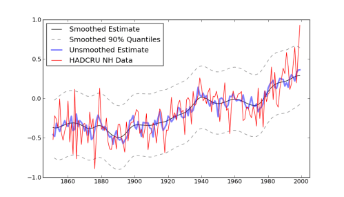
Making an image out of this to match the r version got me stuck for a little bit, because the author snuck in a call to “Friedman’s SuperSmoother” in the plot generation code. That seems unnecessarily sneaky to me, especially after going through all the work of setting up a model with fully bayesian priors. Don’t you want to see the model output before running it through some highly complicated smoothing function? (The super-smoother supsmu is a “running lines smoother which chooses between three spans for the lines”, whatever that is.) In case you do, here it is, together with an alternative smoother I hacked together, since python has no super-smoother that I know of.

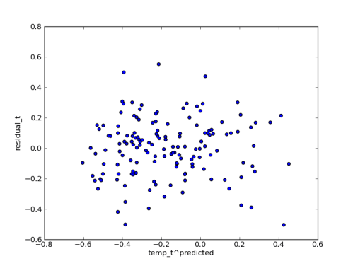
Since I have the posterior predictions handy, I plotted the median residuals against the median predicted temperature values. I think this shows that the error model is fitting the data pretty well:

5 Comments

Filed under MCMC, statistics