MCMC in Python: PyMC for Bayesian Probability

I’ve got an urge to write another introductory tutorial for the Python MCMC package PyMC.  This time, I say enough to the comfortable realm of Markov Chains for their own sake.  In this tutorial, I’ll test the waters of Bayesian probability.

Tom Bayes

Now, what better problem to stick my toe in than the one that inspired Reverend Thomas in the first place? Let’s talk about sex ratio. This is also convenient, because I can crib from Bayesian Data Analysis, that book Rif recommended me a month ago.

Bayes started this enterprise off with a question that has inspired many an evolutionary biologist: are girl children as likely as boy children? Or are they more likely or less likely? Laplace wondered this also, and in his time and place (from 1745 to 1770 in Paris) there were birth records of 241,945 girls and 251,527 boys. In the USA in 2005, the vital registration system recorded 2,118,982 male and 2,019,367 female live births [1]. I’ll set up a Bayesian model of this, and ask PyMC if the sex ratio could really be 1.0.

The simple model of the situation is that there is some number , and every baby flips a biased coin, which says “be a boy” with probability and “be a girl” with probability . This model ignores correlations between twins, the biophysics of sperm, the existence of intersex babies, as well as many other things. All models are wrong, but some are simple examples.

Mathematically, if denotes the number of live births, and denotes the number of boys, the model says

You can think of this as a one parameter model. If I tell the model , then for any and , the model can tell me the probability. Now, to answer a question like “is it possible that ?”, the Bayesians need some sort of prior distribution on . Where does this prior come from? Maybe I should invoke the “principle of insufficient reason”, and say that, since I have no idea, I expect any value between 0 and 1 for , which leads to a uniform distribution on [0,1]. But maybe that’s not an accurate representation of truth; even before I looked up the numbers quoted above, I would have been shocked to learn that , much more shocked than if you told me that . But I’ll hold on to that thought, and go with the uniform prior for now.

In PyMC, it’s 4 lines to set up this model:

from pymc import *
p_b = Uniform('p_b', 0.0, 1.0)
N_b = Binomial('N_b', n=4138349, p=p_b, value=2118982, observed=True)
m = Model([p_b, N_b])

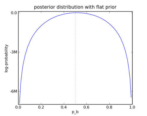
To see the posterior log-probability for a particular value of , do this:

p_b.value = 0.5
print m.logp

Here is the plot:

First Bayesian Example

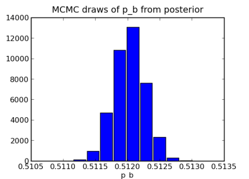
This simple example is so simple that you don’t need any MCMC. But it would be easy to do some if you did.

mc = MCMC(m)
mc.sample(iter=50000,burn=10000)
hist(p_b.trace())

To return to the thought that I’ve been holding, I know that . How can I encode this? I could replace my definition of p_b using something like p_b = Uniform('p_b', 0.0, 0.95), but I’d also be surprised to learn that , so maybe something like p_b = Normal('p_b', 0.5, 0.2) is a good way to go. I don’t know what the pros would think of that; they seem to favor an exotic prior, like p_b = Beta('p_b', 10, 10) which is “conjugate” in this case.

To turn the problem around (and put it in a context I’m familiar with from work), how concentrated does the prior have to be to model a doctor who believes that despite the evidence?

For bonus points, with PyMC we can go beyond the work of Bayes, and model the uncertainty in the vital registration system. These numbers for the USA are probably very close to perfect. But I would be more skeptical of the accuracy for the 241,945 girls and 251,527 boys recorded during Laplace’s day. And how can I represent my skepticism? Maybe I’ll represent it as a normally distributed error with standard deviation 10000.

from pymc import *
p_b = Uniform('p_b', 0.0, 1.0)
e_N = Normal('e_N', 0.0, 1.0/(10000.0)**2)
e_N_b = Normal('e_N_b', 0.0, 1.0/(10000.0)**2)
@potential
def likelihood(N_b=251527, e_N_b=e_N_b, N=241945+251527, e_N=e_N, p=p_b):
    return binomial_like(N_b + e_N_b, N + e_N, p)
mc = MCMC([p_b, N, N_b, likelihood])

Easy, right? Well, easy to write. Can you get PyMC to draw believable samples from it? I can, but it takes a little longer. Remember to thin your samples!