Tag Archives: pymc

Classic EM in Python: Warm-up problem of 197 animals in PyMC

The classic paper on the EM algorithm begins with a little application in multinomial modeling:

Rao (1965, pp. 368-369) presents data in which 197 animals are distributed multinomially into four categories, so that the observed data consist of y = (y_1, y_2, y_3, y_4) = (125, 18, 20, 34).

A genetic model for the population specifies cell probabilities \left(\frac12 + \frac14\pi, \frac14(1-\pi), \frac14(1 -\pi), \frac14\pi\right) for some \pi with 0\leq \pi \leq 1.

Solving this analytically sounds very much like a 1960’s pastime to me (answer: \pi = \frac{15 + \sqrt{53809}}{394}), and a modern computer with PyMC can make short work of numerically approximating this maximum likelihood estimation. It takes no more than this:

import pymc as mc, numpy as np

pi = mc.Uniform('pi', 0, 1)
y = mc.Multinomial('y', n=197, 
                   p=[.5 + .25*pi, .25*(1-pi), .25*(1-pi), .25*pi],
                   value=[125, 18, 20, 34], observed=True)

mc.MAP([pi,y]).fit()
print pi.value

But the point is to warm-up, not to innovate. The EM way is to introduce a latent variable x = (x_1, x_2, x_3, x_4, x_5) and set y_1 = x_1+x_2, y_2=x_3, y_3=x_4, y_4=x_5, and work with a multinomial distribution for x that induces the multinomial distribution above on y. The art is determining a good latent variable, mapping, and distribution, and “good” is meant in terms of the computation it yields:

import pymc as mc, numpy as np

pi = mc.Uniform('pi', 0, 1)

@mc.stochastic
def x(n=197, p=[.5, .25*pi, .25*(1-pi), .25*(1-pi), .25*pi], value=[125.,0.,18.,20.,34.]):
    return mc.multinomial_like(np.round_(value), n, p)

@mc.observed
def y(x=x, value=[125, 18, 20, 34]):
    if np.allclose([x[0]+x[1], x[2], x[3], x[4]], value):
        return 0
    else:
        return -np.inf

It is no longer possible to get a good fit to an mc.MAP object for this model (why?), but EM does not need to. The EM approach is to alternate between two steps:

  • Update x (E-step, because it is set to its conditional expectation based on the current value of \pi)
  • Update \pi (M-step, because it is chosen to maximize the likelihood for the current value of x)

This is simply implemented in PyMC and quick to get the goods:

def E_step():
    x.value = [125 * .5 / (.5 + .25*pi.value), 125 * .25*pi.value / (.5 + .25*pi.value), 18, 20, 34]
def M_step():
    pi.value = (x.value[1] + 34.) / (x.value[1] + 34. + 18. + 20.)
for i in range(5):
    print 'iter %2d: pi=%0.4f, X=%s' %(i, pi.value, x.value)
    E_step()
    M_step()

It is not fair to compare speeds without making both run to the same tolerance, but when that is added EM is 2.5 times faster. That could be important sometimes, I suppose.
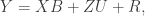
1 Comment

Filed under statistics

MCMC in Python: Bayesian meta-analysis example

In slow progress on my plan to to go through the examples from the OpenBUGS webpage and port them to PyMC, I offer you now Blockers, a random effects meta-analysis of clinical trials.


[py] [pdf]

1 Comment

Filed under MCMC, software engineering

MCMC in Python: A random effects logistic regression example

I have had this idea for a while, to go through the examples from the OpenBUGS webpage and port them to PyMC, so that I can be sure I’m not going much slower than I could be, and so that people can compare MCMC samplers “apples-to-apples”. But its easy to have ideas. Acting on them takes more time.

So I’m happy that I finally found a little time to sit with Kyle Foreman and get started. We ported one example over, the “seeds” random effects logistic regression. It is a nice little example, and it also gave me a chance to put something in the ipython notebook, which I continue to think is a great way to share code.


[py] [pdf]

3 Comments

Filed under MCMC, software engineering

Powell’s Method for Maximization in PyMC

I have been using “Powell’s Method” to find maximum likelihood (ahem, maximum a posteriori) estimates in my PyMC models for years now. It is something that I arrived at by trying all the options once, and it seemed to work most reliably. But what does it do? I never bothered to figure out, until today.

It does something very reasonable. That is to optimize a multidimensional function along one dimension at a time. And it does something very tricky, which is to update the basis for one-dimensional optimization periodically, so that it quickly finds a “good” set of dimensions to optimize over. Now that sounds familiar, doesn’t it? It is definitely the same kind of trick that makes the Adaptive Metropolis step method a winner in MCMC.

The 48-year-old paper introducing the approach, M. J. D. Powell, An efficient method for finding the minimum of a function of several variables without calculating derivatives, is quite readable today. If you want to see it in action, I added an ipython notebook to my pymc examples repository on github: [ipynb] [py] [pdf].

Comments Off on Powell’s Method for Maximization in PyMC

Filed under Uncategorized

Parameterizing Negative Binomial distributions

The negative binomial distribution is cool. Sometimes I think that.

Sometimes I think it is more trouble than it’s worth, a complicated mess.

Today, both.

Wikipedia and PyMC parameterize it differently, and it is a source of continuing confusion for me, so I’m just going to write it out here and have my own reference. (Which will match with PyMC, I hope!)

The important thing about the negative binomial, as far as I’m concerned, is that it is like a Poisson distribution, but “over-dispersed”. That is to say that the standard deviation is not always the square root of the mean. So I’d like to parameterize it with a parameter \mu for the mean and \delta for the dispersion. This is almost what PyMC does, except it calls the dispersion parameter \alpha instead of \delta.

The slightly less important, but still informative, thing about the negative binomial, as far as I’m concerned, is that the way it is like a Poisson distribution is very direct. A negative binomial is a Poisson that has a Gamma-distributed random variable for its rate. In other words (symbols?), Y \sim \text{NegativeBinomial}(\mu, \delta) is just shorthand for

Y \sim \text{Poisson}(\lambda),
\lambda \sim \text{Gamma}(\mu, \delta).

Unfortunately, nobody parameterizes the Gamma distribution this way. And so things get really confusing.

The way to get unconfused is to write out the distributions, although after they’re written, you might doubt me:

The negative binomial distribution is
f(k \mid \mu, \delta) = \frac{\Gamma(k+\delta)}{k! \Gamma(\delta)} (\delta/(\mu+\delta))^\delta (\mu/(\mu+\delta))^k
and the Poisson distribution is
f(k \mid \lambda) = \frac{e^{-\lambda}\lambda^k}{k!}
and the Gamma distribution is
f(x \mid \alpha, \beta) = \frac{\beta^{\alpha}x^{\alpha-1}e^{-\beta x}}{\Gamma(\alpha)}

Hmm, does that help yet? If \alpha = \delta and \beta = \delta/\mu, it all works out:
\frac{\Gamma(k+\delta)}{\Gamma(\delta)k!} \left(\frac{\delta}{\pi+\delta}\right)^\delta \left(\frac{\pi}{\pi+\delta}\right)^k  =  \int_0^\infty \frac{e^{-\lambda}\lambda^k}{k!} \lambda^{\delta-1} e^{-\lambda \delta/\mu} \frac{(\delta/\mu)^{\delta}}{\Gamma(\delta)}d \lambda.

But instead of integrating it analytically (or in addition to), I am extra re-assured by seeing the results of a little PyMC model for this:

I put a notebook for making this plot in my pymc-examples repository. Love those notebooks. [pdf] [ipynb]

1 Comment

Filed under statistics

PyMC+Pandas: Poisson Regression Example

When I was gushing about the python data package pandas, commenter Rafael S. Calsaverini asked about combining it with PyMC, the python MCMC package that I usually gush about. I had a few minutes free and gave it a try. And just for fun I gave it a try in the new ipython notebook. It works, but it could work even better. See attached:

[pdf] [ipynb]

3 Comments

Filed under MCMC, software engineering

Causal Modeling in Python: Bayesian Networks in PyMC

While I was off being really busy, an interesting project to learn PyMC was discussed on their mailing list, beginning thusly:

I am trying to learn PyMC and I decided to start from the very simple discrete Sprinkler model.
I have found plenty of examples for continuous models, but I am not sure how should I proceed with conditional tables, especially when the condition is over more than a variable. How would you model a CPT with PyMC, and in particular the Sprinkler model?

I spend all my time on continuous models these days, and I miss my old topics from back in grad school. Not that this is one of them, exactly. But when I found myself with a long wait while running some validation code, I thought I’d give it a try. The model turned out to be simple, although using MCMC to fit it is probably not the best idea. Continue reading

2 Comments

Filed under MCMC

PyMC at SciPy 2011

I just returned from the SciPy 2011 conference in Austin. Definitely a different experience than a theory conference, and definitely different than the mega-conferences I’ve found myself at lately. I think I like it. My goal was to evangelize for PyMC a little bit, and I think that went successfully. I even got to meet PyMC founder Chris Fonnesbeck in person (about 30 seconds before we presented a 4 hour tutorial together).

For the tutorial, I put together a set of PyMC-by-Example slides and code to dig into that silly relationship between Human Development Index and Total Fertility Rate that foiled my best attempts at Bayesian model selection so long ago.

I’m not sure the slides stand on their own, but together with the code samples they should reproduce my portion of the talk pretty well. I even started writing it up for people who want to read it in paper form, but then I ran out of momentum. Patches welcome.

Comments Off on PyMC at SciPy 2011

Filed under education, global health, MCMC, statistics

My First Contribution to PyMC

I’m excited to report that my first contribution back to the PyMC codebase was accepted. 🙂

It is a slight reworking of the pymc.Matplot.plot function that make it include autocorrelation plots of the trace, as well as histograms and timeseries.  I also made the histogram look nicer (in my humble opinion).

Before:

After:

In this example, I can tell that MCMC hasn’t converged from the trace of beta_2 without my changes, but it is dead obvious from the autocorrelation plot of beta_2 in the new version.

The process of making changes to the pymc sourcecode is something that has intimidated me for a while.  Here are the steps in my workflow, in case it helps you get started doing this, too.

# first fork a copy of pymc from https://github.com/pymc-devs/pymc.git on github
git clone https://github.com/pymc-devs/pymc.git

# then use virtualenv to install it and make sure the tests work
virtualenv env_pymc_dev
source env_pymc_dev/bin/activate

# then you can install pymc without being root
cd pymc
python setup.py install
# so you can make changes to it without breaking everything else

# to test that it is working
cd ..
python
>>> import pymc
>>> pymc.test()
# then make changes to pymc...
# to test changes, and make sure that all of the tests that use to pass still do repeat the process above
cd pymc
python setup.py install
cd ..
python
>>> import pymc
>>> pymc.test()

# once everything is perfect, push it to a public git repo and send a "pull request" to the pymc developers.

Is there an easier way?  Let me know in the comments.

1 Comment

Filed under MCMC, software engineering

MCMC in Python: A simple random effects model and its extensions

A nice example of using PyMC for multilevel (aka “Random Effects”) modeling came through on the PyMC mailing list a couple of weeks ago, and I’ve put it into a git repo so that I can play around with it a little, and collect up the feedback that the list generates.

Here is the situation:

Hi All,

New to this group and to PyMC (and mostly new to Python). In any case, I’m writing to ask for help in specifying a multilevel model (mixed model) for what I call partially clustered designs. An example of a partially clustered design is a 2-condition randomized psychotherapy study where subjects are randomly assigned to conditions. In condition 1, subjects are treated in small groups of say 8 people a piece. In the condition 2, usually a control, subjects are only assessed on the outcome (they don’t receive an intervention). Thus you have clustering in condition 1 but not condition 2.

The model for a 2-condition study looks like (just a single time point to keep things simpler):
y_{ij} = b_0 + b_1 Tx + u_j Tx + e_{ij},
where y_ij is the outcome for the ith person in cluster j (in most multilevel modeling software and in PROC MCMC in SAS, subjects in the unclustered condition are all in clusters of just 1 person), b_0 is the overall intercept, b_1 is the treatment effect, Tx is a dummy coded variable coded as 1 for the clustered condition and 0 for the unclustered condition, u_j is the random effect for cluster j, and e_ij is the residual error. The variance among clusters is \sigma^2_u and the residual term is \sigma^2_e (ideally you would estimate a unique residual by condition).

Because u_j interacts with Tx, the random effect is only contributes to the clustered condition.

In my PyMC model, I expressed the model in matrix form – I find it easier to deal with especially for dealing with the cluster effects. Namely:
Y = XB + ZU + R,
where X is an n x 2 design matrix for the overall intercept and intervention effect, B is a 1 x 2 matrix of regression coefficients, Z is an n x c design matrix for the cluster effects (where c is equal to the number of clusters in the clustered condition), and U is a c x 1 matrix of cluster effects. The way I’ve written the model below, I have R as an n x n diagonal matrix with \sigma^2_e on the diagonal and 0’s on the off-diagonal.

All priors below are based on a model fit in PROC MCMC in SAS. I’m trying to replicate the analyses in PyMC so I don’t want to change the priors.

The data consist of 200 total subjects. 100 in the clustered condition and 100 in the unclustered. In the clustered condition there are 10 clusters of 10 people each. There is a single outcome variable.

I have 3 specific questions about the model:

  1. Given the description of the model, have I successfully specified the model? The results are quite similar to PROC MCMC, though the cluster variance (\sigma^2_u) differs more than I would expect due to Monte Carlo error. The differences make me wonder if I haven’t got it quite right in PyMC.
  2. Is there a better (or more efficient) way to set up the model? The model runs quickly but I am trying to learn Python and to get better at optimizing how to set up models (especially multilevel models).
  3. How can change my specification so that I can estimate unique residual variances for clustered and unclustered conditions? Right now I’ve estimated just a single residual variance. But I typically want separate estimates for the residual variances per intervention condition.

Here are my first responses:

1. This code worked for me without any modification. 🙂 Although when
I tried to run it twice in the same ipython session, it gave me
strange complaints. (for pymc version 2.1alpha, wall time 78s).
For the newest version in the git repo (pymc version 2.2grad,
commit ca77b7aa28c75f6d0e8172dd1f1c3f2cf7358135, wall time 75s) it
didn’t complain.

2. I find the data wrangling section of the model quite opaque. If
there is a difference between the PROC MCMC and PyMC results, this
is the first place I would look. I’ve been searching for the most
transparent ways to deal with data in Python, so I can share some
of my findings as applied to this block of code.

3. The model could probably be faster. This is the time for me to
recall the two cardinal rules of program optimization: 1) Don’t
Optimize, and 2) (for experts only) Don’t Optimize Yet.

That said, the biggest change to the time PyMC takes to run is in
the step methods. But adjusting this is a delicate operation.
More on this to follow.

4. Changing the specification is the true power of the PyMC approach,
and why this is worth the extra effort, since a random effects
model like yours is one line of STATA. So I’d like to write out
in detail how to change it. More on this to follow.

5. Indentation should be 4 spaces. Diverging from this inane detail
will make python people itchy.

Have a look in the revision history and the git repo README for more.

Good times. Here is my final note from the time I spent messing around:
Django and Rails have gotten a lot of mileage out of emphasizing
_convention_ in frequently performed tasks, and I think that PyMC
models could also benefit from this approach. I’m sure I can’t
develop our conventions myself, but I have changed all the file names
to move towards what I think we might want them to look like. Commit
linked here
.

My analyses often have these basic parts: data, model, fitting code,
graphics code. Maybe your do, too.

p.s. Scott and I have started making an automatic model translator, to generate models like this from the kind of concise specification that users of R and STATA are familiar with. More news on that in a future post.

1 Comment

Filed under MCMC, statistics