Tag Archives: python

MCMC in Python: A simple random effects model and its extensions

A nice example of using PyMC for multilevel (aka “Random Effects”) modeling came through on the PyMC mailing list a couple of weeks ago, and I’ve put it into a git repo so that I can play around with it a little, and collect up the feedback that the list generates.

Here is the situation:

Hi All,

New to this group and to PyMC (and mostly new to Python). In any case, I’m writing to ask for help in specifying a multilevel model (mixed model) for what I call partially clustered designs. An example of a partially clustered design is a 2-condition randomized psychotherapy study where subjects are randomly assigned to conditions. In condition 1, subjects are treated in small groups of say 8 people a piece. In the condition 2, usually a control, subjects are only assessed on the outcome (they don’t receive an intervention). Thus you have clustering in condition 1 but not condition 2.

The model for a 2-condition study looks like (just a single time point to keep things simpler):
y_{ij} = b_0 + b_1 Tx + u_j Tx + e_{ij},
where y_ij is the outcome for the ith person in cluster j (in most multilevel modeling software and in PROC MCMC in SAS, subjects in the unclustered condition are all in clusters of just 1 person), b_0 is the overall intercept, b_1 is the treatment effect, Tx is a dummy coded variable coded as 1 for the clustered condition and 0 for the unclustered condition, u_j is the random effect for cluster j, and e_ij is the residual error. The variance among clusters is \sigma^2_u and the residual term is \sigma^2_e (ideally you would estimate a unique residual by condition).

Because u_j interacts with Tx, the random effect is only contributes to the clustered condition.

In my PyMC model, I expressed the model in matrix form – I find it easier to deal with especially for dealing with the cluster effects. Namely:
Y = XB + ZU + R,
where X is an n x 2 design matrix for the overall intercept and intervention effect, B is a 1 x 2 matrix of regression coefficients, Z is an n x c design matrix for the cluster effects (where c is equal to the number of clusters in the clustered condition), and U is a c x 1 matrix of cluster effects. The way I’ve written the model below, I have R as an n x n diagonal matrix with \sigma^2_e on the diagonal and 0’s on the off-diagonal.

All priors below are based on a model fit in PROC MCMC in SAS. I’m trying to replicate the analyses in PyMC so I don’t want to change the priors.

The data consist of 200 total subjects. 100 in the clustered condition and 100 in the unclustered. In the clustered condition there are 10 clusters of 10 people each. There is a single outcome variable.

I have 3 specific questions about the model:

  1. Given the description of the model, have I successfully specified the model? The results are quite similar to PROC MCMC, though the cluster variance (\sigma^2_u) differs more than I would expect due to Monte Carlo error. The differences make me wonder if I haven’t got it quite right in PyMC.
  2. Is there a better (or more efficient) way to set up the model? The model runs quickly but I am trying to learn Python and to get better at optimizing how to set up models (especially multilevel models).
  3. How can change my specification so that I can estimate unique residual variances for clustered and unclustered conditions? Right now I’ve estimated just a single residual variance. But I typically want separate estimates for the residual variances per intervention condition.

Here are my first responses:

1. This code worked for me without any modification. 🙂 Although when
I tried to run it twice in the same ipython session, it gave me
strange complaints. (for pymc version 2.1alpha, wall time 78s).
For the newest version in the git repo (pymc version 2.2grad,
commit ca77b7aa28c75f6d0e8172dd1f1c3f2cf7358135, wall time 75s) it
didn’t complain.

2. I find the data wrangling section of the model quite opaque. If
there is a difference between the PROC MCMC and PyMC results, this
is the first place I would look. I’ve been searching for the most
transparent ways to deal with data in Python, so I can share some
of my findings as applied to this block of code.

3. The model could probably be faster. This is the time for me to
recall the two cardinal rules of program optimization: 1) Don’t
Optimize, and 2) (for experts only) Don’t Optimize Yet.

That said, the biggest change to the time PyMC takes to run is in
the step methods. But adjusting this is a delicate operation.
More on this to follow.

4. Changing the specification is the true power of the PyMC approach,
and why this is worth the extra effort, since a random effects
model like yours is one line of STATA. So I’d like to write out
in detail how to change it. More on this to follow.

5. Indentation should be 4 spaces. Diverging from this inane detail
will make python people itchy.

Have a look in the revision history and the git repo README for more.

Good times. Here is my final note from the time I spent messing around:
Django and Rails have gotten a lot of mileage out of emphasizing
_convention_ in frequently performed tasks, and I think that PyMC
models could also benefit from this approach. I’m sure I can’t
develop our conventions myself, but I have changed all the file names
to move towards what I think we might want them to look like. Commit
linked here
.

My analyses often have these basic parts: data, model, fitting code,
graphics code. Maybe your do, too.

p.s. Scott and I have started making an automatic model translator, to generate models like this from the kind of concise specification that users of R and STATA are familiar with. More news on that in a future post.

1 Comment

Filed under MCMC, statistics

Data Wrangling in R, Stata and Python

It was nearly a year ago when I was accosted by students I had urged to try Python and their complaints that the data manipulation capabilities they found so convenient in R and Stata were nowhere to be found. At the time, I did some digging and told them to try la.larry (or pandas, as mentioned by readers of that post). With some more experience, these recommendations have come up again, and in hindsight it seems like la.larry is too heavy a hammer for our most common tasks.

I’m hoping to put together a translation guide for R, Stata, and Python (there is already an extensive one… ours will be much more specialized, to just a few data wrangling commands), and until then, here are Kyle’s top two:

The easiest way to build record arrays (aside from csv2rec) IMO:

import numpy as np
a = ['USA','USA','CAN']
b = [1,6,4]
c = [1990.1,2005.,1995.]
d = ['x','y','z']
some_recarray = np.core.records.fromarrays([a,b,c,d], names=['country','age','year','data'])

The fromarrays method is especially nice because it automatically deals with datatypes.

To subset a particular country-year-age:

some_recarray[(some_recarray.country=='USA')
                & (some_recarray.age==6)
                & (some_recarray.year==2005)]

I’ve also found that caching each of the indices independently vastly speeds things up if you’re going to be iterating.

Love the recarray, hate the documentation.

6 Comments

Filed under software engineering

Introducing the H-RAM

I haven’t had time to say much recently, due to some travel for work, but I did have a chance to prototype the Hit-and-Run/Adaptive Metropolis approach to MCMC that I mentioned in my last post.  Was that really three weeks ago?  How time flies.

Anyway, thanks to the tip Aram pointed out in the comments, Hit-and-Run can take steps in the correct direction without explicitly computing an approximation of the covariance matrix, just by taking a randomly weighted sum of random points.  It’s nearly magic, although Aram says that it actually makes plenty of sense. The code for this “H-RAM” looks pretty similar to my original Hit-and-Run step method, and it’s short enough that I’ll just show it to you:

class HRAM(Gibbs):
    def __init__(self, stochastic, proposal_sd=None, verbose=None):
        Metropolis.__init__(self, stochastic, proposal_sd=proposal_sd,
                            verbose=verbose, tally=False)
        self.proposal_tau = self.proposal_sd**-2.
        self.n = 0
        self.N = 11
        self.value = rnormal(self.stochastic.value, self.proposal_tau, size=tuple([self.N] + list(self.stochastic.value.shape)))

    def step(self):
        x0 = self.value[self.n]
        u = rnormal(zeros(self.N), 1.)
        dx = dot(u, self.value)

        self.stochastic.value = x0
        logp = [self.logp_plus_loglike]
        x_prime = [x0]

        for direction in [-1, 1]:
            for i in xrange(25):
                delta = direction*exp(.1*i)*dx
                try:
                    self.stochastic.value = x0 + delta
                    logp.append(self.logp_plus_loglike)
                    x_prime.append(x0 + delta)
                except ZeroProbability:
                    self.stochastic.value = x0

        i = rcategorical(exp(array(logp) - flib.logsum(logp)))
        self.value[self.n] = x_prime[i]
        self.stochastic.value = x_prime[i]

        if i == 0:
            self.rejected += 1
        else:
            self.accepted += 1

        self.n += 1
        if self.n == self.N:
            self.n = 0

Compare the results to the plain old Hit-and-Run step method:

9 Comments

Filed under MCMC

MCMC in Python: Custom StepMethods and bounded-depth spanning tree distraction

I was looking for a distraction earlier this week, which led me to the world of stackexchange sites. The stack overflow has been on my radar for a while now, because web-search for coding questions often leads there and the answers are often good. And I knew that math overflow, tcs overflow, and even stats overflow existed, but I’d never really explored these things.

Well, diversion found! I got enamored with an MCMC question on the tcs site, about how to find random bounded-depth spanning trees. Bounded-depth spanning trees are something that I worked on with David Wilson and Riccardo Zechinna in my waning days of my MSR post-doc, and we came up with some nice results, but the theoretical ones are just theory, and the practical ones are based on message passing algorithms that still seem magical to me, even after hours of patient explanation from my collaborators.

So let’s do it in PyMC… this amounts to an exercise in writing custom step methods, something that’s been on my mind for a while anyways. And, as a bonus, I got to make an animation of the chain in action which I find incredibly soothing to watch on repeat:

Continue reading

3 Comments

Filed under MCMC, TCS

Beautiful Networks

I’ve had a secret project running in the background this week two weeks ago (how time flies!), a continuation of my work on bias reduction for traceroute sampling. It would be nice if this had applications to global health, but unfortunately (and uncharacteristically) I can’t think of any. It is a great opportunity for visualizing networks, though, a topic worthy of a quick post.

The bowl-of-spaghetti network visualization has been a staple of complex networks research for the last decade. I’m not convinced that there is anything interesting to learn from real world networks by drawing them in 2 or 3 dimensions, but the graphics a seriously eye catching. And I’m not convinced that there isn’t anything to learn from them, either. I invite you to convince me in the comments.

Interesting?


What my side project has reminded me of, however, is the value of drawing networks in 2 dimensions for illustrating the principles of network algorithms and network statistics. And if the topic of study is complex or real-world or random networks, than a little bit of spaghetti in the graphic seems appropriate.

There are a lot of nice tools for doing this now, and just collecting the things I should consider in one place makes this post worthwhile for me. I learn towards a Pythonic solution of networkx driving graphviz, but there are some javascript options out there now that seem promising (jit, protovis, possibly more from a stackoverflow question) in. And for those looking for a less command-line-based solution, the Pajek system seems like a good route.

As for what to graph, here are my thoughts. The Erdos-Renyi graph doesn’t look good, and the Preferential Attachment graph doesn’t look good. Use them for your theorems and for your simulations, but when it comes time to draw something, consider a random geometric graph. And since these can be a little dense, you might want an “edge-percolated random geometric graph”.

I did have a little trouble with this approach, too, when I was drawing minimum spanning trees, because the random geometric points end up being placed really close together occasionally. So maybe the absolutely best random graph for illustrations would be a geometric graph with vertices from a “hard core” model, which is to say random conditioned on being a minimum distance apart. Unfortunately, it is an open question how to efficiently generate hard-core points. But it’s not hard to fake:

More informative?


Want some of your own? Here’s the code.

Comments Off on Beautiful Networks

Filed under probability

Nice post on Cython

Python/Sage guru William Stein has a nice article about Cython and how it can speed up routine calculations at the expense of mathematical elegance (and why that is a good thing). Could Sage be my interactive shell for PyMC modeling?

Comments Off on Nice post on Cython

Filed under software engineering

MCMC in Python: Global Temperature Reconstruction with PyMC

A short note on the PyMC mailing list alerted me that the Apeescape, the author of mind of a Markov chain blog, was thinking of using PyMC for replicating some controversial climate data analysis, but was having problems with it. Since I’m a sucker for controversial data, I decided to see if I could do the replication exercise in PyMC myself.

I didn’t dig in to what the climate-hockey-stick fuss is about, that’s something I’ll leave for my copious spare time. What I did do is find the data pretty easily available on the original author’s website, and make a translation of the R/bugs model into pymc/python. My work is all in a github repository if you want to try it yourself, here.

Based on Apeescape’s bugs model, I want to have \textnormal{temp}_t = N(\mu_t, \sigma^2) where \mu_t = \beta_0 + \beta_1\textnormal{temp}_{t-1} + \beta_2\textnormal{temp}_{t-2} + \sum_{i=3}^{12} \beta_i(\textnormal{PC})_{t,i}, with priors \vec{\beta} \sim N(\vec{0}, 1000 I) and \sigma \sim \textnormal{Uniform}(0,100).

I implemented this in a satisfyingly concise 21 lines of code, that also generate posterior predictive values for model validation:

# load data                                                                                                                                                                      
data = csv2rec('BUGS_data.txt', delimiter='\t')


# define priors                                                                                                                                                                  
beta = Normal('beta', mu=zeros(13), tau=.001, value=zeros(13))
sigma = Uniform('sigma', lower=0., upper=100., value=1.)


# define predictions                                                                                                                                                             
pc = array([data['pc%d'%(ii+1)] for ii in range(10)]) # copy pc data into an array for speed & convenience                                                                       
@deterministic
def mu(beta=beta, temp1=data.lagy1, temp2=data.lagy2, pc=pc):
    return beta[0] + beta[1]*temp1 + beta[2]*temp2 + dot(beta[3:], pc)

@deterministic
def predicted(mu=mu, sigma=sigma):
    return rnormal(mu, sigma**-2.)

# define likelihood                                                                                                                                                              
@observed
def y(value=data.y, mu=mu, sigma=sigma):
    return normal_like(value, mu, sigma**-2.)

Making an image out of this to match the r version got me stuck for a little bit, because the author snuck in a call to “Friedman’s SuperSmoother” in the plot generation code. That seems unnecessarily sneaky to me, especially after going through all the work of setting up a model with fully bayesian priors. Don’t you want to see the model output before running it through some highly complicated smoothing function? (The super-smoother supsmu is a “running lines smoother which chooses between three spans for the lines”, whatever that is.) In case you do, here it is, together with an alternative smoother I hacked together, since python has no super-smoother that I know of.

Since I have the posterior predictions handy, I plotted the median residuals against the median predicted temperature values. I think this shows that the error model is fitting the data pretty well:

5 Comments

Filed under MCMC, statistics

MCMC in Python: Sudoku is a strange game

I was on a “vacation” for the last week, which included a real vacation to visit my parents, and also a scare-quotes vacation to Detroit that is a totally different subject. But the side effect of this vacation that is to be the topic of this post is the strange game of Sudoku, which is popular with travelers.

Jessi was with me and she seems to like this Sudoku business (although she denies it), so I thought about playing, too. But I always get interested in the wrong parts of these games. Solving Sudoku puzzles seems more like a game for computers than humans, and writing a program to let computers have their fun is the way I would prefer to waste time while en route. There really isn’t much to it:

def solve(T):
    # if all cells are filled in, we win
    if all(T > 0):
        return 'success'

    # solve T recursively, by trying all values for the most constrained var
    pos = possibilities(T)
    i,j = most_constrained(T, pos)

    for val in pos[(i,j)]:
        T[i,j] = val
        if solve(T) == 'success':
            return 'success'

    # if this point is reached, this branch is unsatisfiable
    T[i, j] = -1
    return 'failure'

Is this ruining anyone’s homework problems? Just in case it is, everything I said at the beginning of my post on minimum spanning trees still applies.

With plenty of time left in my flight, this was just the opening move, though. The real question is what makes this fun for the humans who find this kind of thing fun? One hypothesis, the kind that comes naturally when you have watched the statistical physicists in action, is that fun is some sort of phase transition, and if you take random Sudoku puzzles with a certain number of entries you will maximize fun. Half-baked, I know, but as interesting as the movies they show on planes, at least. And it raises the extremely important, and possibly unsolved challenge, how do you sample uniformly at random from Sudoku puzzles with n cells filled in?

In my travel-addled state, I thought maybe a good way to do it would be to start with some complete configuration, knockout a large fraction of the cells at random, permute the remaining cells, and then solve the resulting configuration. Repeating this has got to be an ergodic markov chain, right? I’m not sure… and even then, do you think the stationary distribution is uniform?

def rand(n, T=None):
    # start with an empty board
    if T == None:
        T = -1*ones([9,9])

    # solve it to generate an initial solution
    solve(T)

    # do random shuffles to approximate uniformly random solution
    for k in range(5):
        select_random_cells(T, 20)
        randomly_permute_labels(T)
        solve(T)

    # remove appropriate amount of labels
    select_random_cells(T, n)

    return T

Now, when Jessi found out that I was helping computers take her sudoku-solving job away, she thought I was a geek, but when she found out I was generating puzzles with more than one solution, she was outraged. Sudoku puzzles have a unique solution! So maybe what is really fun is a random puzzle with a unique solution, and the right number of cells filled in, where a smaller number of cells means that harder puzzles are right. Fortunately/unfortunately my travel ended before I finished investigating this important issue.

I doubt it is related, but I got pretty sick the next day.

8 Comments

Filed under MCMC

la.larry for classy number crunching in Python

I’ve got some of my colleagues interested in using Python to cruch their numbers, and that’s great, because I’m sure it will make their lives much better in the long run. It’s also great because they are pushing me to figure out the easy way to do things, since they are used to certain conveniences from their past work with R and STATA.

For example, Kyle wanted to know does Python make it easy to deal with the tables of data he is faced with every day?

It was by showing my ignorance in a blog post a year ago that I learned about handing csv files with the csv.DictReader class. And this has been convenient enough for me, but it doesn’t let Kyle do the things the way he is used to, for example using data[[‘iso3’, ‘gdp’], :] to select these two important columns from a large table.

Enter larry, the labeled array. Maybe someone will tell me an even cleaner way to deal with these tables, but after a quick easy_install la, I was able to load up some data from the National Cancer Institute (NCI) as follows:

import csv
import la
from pylab import *

csv_file = csv.reader(open('accstate5.txt'))
columns = csv_file.next()[1:]
rows = []
data = []

for d in csv_file:
    rows.append(d[0])
    data.append(d[1:])

T = la.larry(data, [rows, columns])

That’s pretty good, but the data is not properly coded as floating point…

T = la.larry(data, [rows, columns]).astype(float)

Now, T has the whole table, indexed by state and by strange NCI code

T.lix[['WA', 'OR', 'ID', 'MO'], ['RBM9094']]

Perfect, besides being slightly ugly. But is there an easier way? the la documentation mentions a fromcsv method. Unfortunately la.larry.fromcsv doesn’t like these short-format tables.

la.larry.fromcsv('accstate5.txt')  # produces a strange error

Now, if you read the NCI data download info page, where I retrieved this data from, you will learn what each cryptic column heading means:

Column heading format:   [V] [RG] [T] [A], where

V = variable: R, C, LB, or UB
RG = race / gender: BM, BF, WM, WF (B = black, W = white, F = female, M = male)
T = calendar time: 5094, 5069, 7094, and the 9 5-year periods 5054 through 9094
A = age group: blank (all ages), 019, 2049, 5074, 75+

Example:
RBM5054 = rate for black males for the time period 1950-1954

That means I’m not really dealing with a 2-dimensional table after all, and maybe I’d be better off organizing things the way they really
are:

data_dict_list = [d for d in csv.DictReader(open('accstate5.txt'))]
data_dict = {}
races = ['B', 'W']
sexes = ['M', 'F']
times = range(50,95,5)
for d in data_dict_list:
    for race in races:
        for sex in sexes:
            for time in times:
                key = 'R%s%s%d%d' % (race, sex, time, time+4)
                val = float(d.get(key, nan)) # larry uses nan to denote missingdata
                data_dict[(d['STATE'], race, sex, '19%s'%time)] = val

R = la.larry.fromdict(data_dict)

In the original 2-d labeled array we can compare cancer rates thusly:

states = ['OR', 'WA', 'ID', 'MT']
times = arange(50,94,5)
selected_cols = ['RWM%d%d' % (t, t+4) for t in times]
T_selected = T.lix[states, selected_cols]
plot(1900+times, T_selected.getx().T, 's-',
     linewidth=3, markersize=15, alpha=.75)
legend(T_selected.getlabel(0), loc='lower right', numpoints=3, markerscale=.5)
ylabel('Mortality rate (per 100,000 person-years)')
xlabel('Time (years)')
title('Mortality rate for all cancers over time')
axis([1945, 1995, 0, 230])

It is slightly cooler to do the same plot with the multi-dimensional array

clf()
subplot(2,1,1)

times = [str(t) for t in range(1950, 1994, 5)]
states = ['OR', 'WA', 'ID', 'MT']
colors = ['c', 'b', 'r', 'g']
for state, color in zip(states, colors):
    plot(R.getlabel(3), R.lix[[state], ['W'], ['M'], :].getx(), 's-', color=color,
         linewidth=3, markersize=15, alpha=.75)
legend(T_selected.getlabel(0), loc='lower right', numpoints=3, markerscale=.5)
ylabel('Mortality rate (per 100,000 person-years)')
xlabel('Time (years)')
title('Mortality rate for all cancers in white males over time')
axis([1945, 1995, 0, 230])

That should be enough for me to remember how to use larry when I come back to it in the future. For my final trick, let’s explore how to use larrys to add a column to a 2-dimensional table. (There is some important extension of this to multidimensional tables, but it is confusing me a lot right now.)

states = T.getlabel(0)
X = la.larry(randn(len(states), 1), [states, ['new covariate']])
T = T.merge(X)

states = ['OR', 'WA', 'ID', 'MT']
T.lix[states, ['RWM9094', 'new covariate']]

Ok, encore… how well does larry play with PyMC? Let’s use a Gaussian Process model to find out.

from pymc import *

M = gp.Mean(lambda x, mu=R.mean(): mu * ones(len(x)))
C = gp.Covariance(gp.matern.euclidean, diff_degree=2., amp=1., scale=1.)
mesh = array([[i,j,k,.5*l] for i in range(52) for j in range(2) for k in range(2) for l in arange(9)])

obs_mesh = array([[i,j,k,.5*l] for i in range(52) for j in range(2) for k in range(2) for l in range(9) if not isnan(R[i,j,k,l])])
obs_vals = array([R[i,j,k,l] for i in range(52) for j in range(2) for k in range(2) for l in range(9) if not isnan(R[i,j,k,l])])
obs_V = array([1. for i in range(52) for j in range(2) for k in range(2) for l in range(9) if not isnan(R[i,j,k,l])])

gp.observe(M, C, obs_mesh, obs_vals, obs_V)
imputed_vals = M(mesh)
imputed_std = sqrt(abs(C(mesh)))

Ri = la.larry(imputed_vals.reshape(R.shape), R.label)

subplot(2,1,2)
for state, color in zip(states, colors):
    t = [float(l) for l in Ri.getlabel(3)]
    plot(t, R.lix[[state], ['B'], ['M'], :].getx(), '^', color=color, linewidth=3, markersize=15, alpha=.75)
    plot(t, Ri.lix[[state], ['B'], ['M'], :].getx(), '-', color=color, linewidth=2, alpha=.75)

ylabel('Mortality rate (per 100,000 person-years)')
xlabel('Time (years)')
title('Mortality rate for all cancers in black males over time')
axis([1945, 1995, 0, 630])
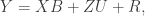
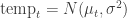
5 Comments

Filed under software engineering

Random Graphs in NetworkX: My Spatial-Temporal Preferred Attachment Diversion

To take my mind off my meetings, I spent a little time modifying the Spatial Preferred Attachment model from Aiello, Bonato, Cooper, Janssen, and PraÅ‚at’s paper A Spatial Web Graph Model with Local Influence Regions so that it changes over time. Continue reading

3 Comments

Filed under combinatorics, probability